ベイジアン構造化時系列モデルは任意の観測時系列データの構造上の継承について学習する興味深い方法です。それはまた私たちに予測問題について別な視点を与える将来を推測するための暗黙の予測分布を作る能力を与えます。私たちは、同じ尺度でまだ実現していない将来の状態の構造に関する情報として、これまで観察した時系列データの学習済みの特徴をとり扱うことができます。
このノートブックでは自己回帰構造の時系列データの範囲を予測することと、そして重要なこととしてモデルの将来の観測値の予測の方法と、適合の方法を見ていきます。
import arviz as az
import numpy as np
import pandas as pd
import pymc as pm

from matplotlib import pyplot as plt
RANDOM_SEED = 8929
rng = np.random.default_rng(RANDOM_SEED)
az.style.use("arviz-darkgrid")フェイク自己回帰データの生成
最初に簡単な自己回帰時系列を生成します。私たちはモデルを決定しこのデータを適合する方法をお見せし、その後、データに幾つかの複雑性を追加し、如何にして自己回帰モデルに取り込めるか、未来のシェイプの予測の仕方についてお見せしましょう。
def simulate_ar(intercept, coef1, coef2, noise=0.3, *, warmup=10, steps=200):
    # We sample some extra warmup steps, to let the AR process stabilize
    draws = np.zeros(warmup + steps)
    # Initialize first draws at intercept
    draws[:2] = intercept
    for step in range(2, warmup + steps):
        draws[step] = (
            intercept
            + coef1 * draws[step - 1]
            + coef2 * draws[step - 2]
            + np.random.normal(0, noise)
        )
    # Discard the warmup draws
    return draws[warmup:]


# True parameters of the AR process
ar1_data = simulate_ar(10, -0.9, 0)

fig, ax = plt.subplots(figsize=(10, 3))
ax.set_title("Generated Autoregressive Timeseries", fontsize=15)
ax.plot(ar1_data);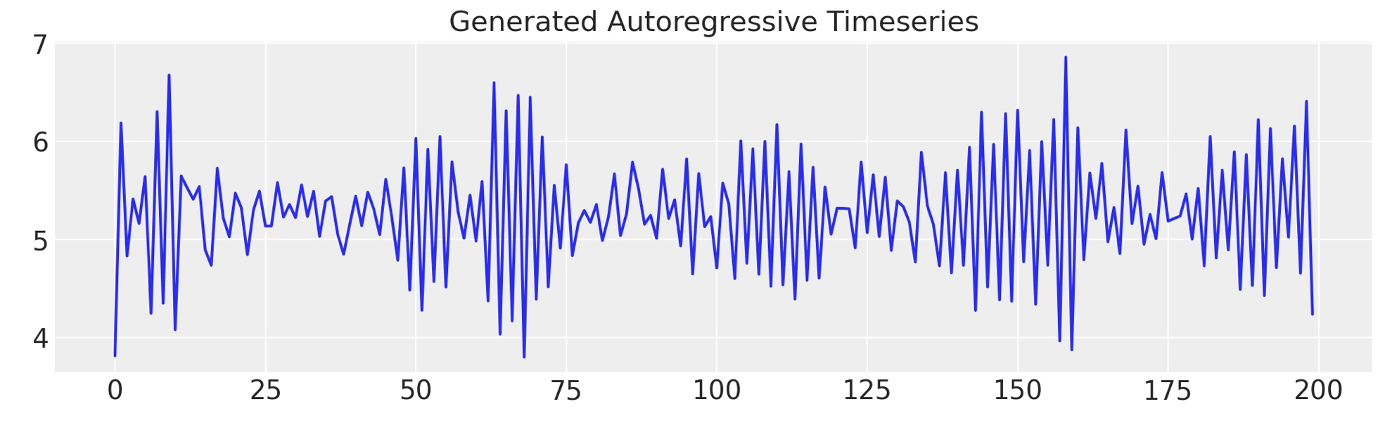
モデルの詳細規定
モデルを順番に進んでいきます。そしてパターンを、複雑な構造の成分の組み合わせを増加させて利用することができる関数に一般化します。
## Set up a dictionary for the specification of our priors
## We set up the dictionary to specify size of the AR coefficients in
## case we want to vary the AR lags.
priors = {
    "coefs": {"mu": [10, 0.2], "sigma": [0.1, 0.1], "size": 2},
    "sigma": 8,
    "init": {"mu": 9, "sigma": 0.1, "size": 1},
}

## Initialise the model
with pm.Model() as AR:
    pass

## Define the time interval for fitting the data
t_data = list(range(len(ar1_data)))
## Add the time interval as a mutable coordinate to the model to allow for future predictions
AR.add_coord("obs_id", t_data, mutable=True)

with AR:
    ## Data containers to enable prediction
    t = pm.MutableData("t", t_data, dims="obs_id")
    y = pm.MutableData("y", ar1_data, dims="obs_id")

    # The first coefficient will be the constant term but we need to set priors for each coefficient in the AR process
    coefs = pm.Normal("coefs", priors["coefs"]["mu"], priors["coefs"]["sigma"])
    sigma = pm.HalfNormal("sigma", priors["sigma"])
    # We need one init variable for each lag, hence size is variable too
    init = pm.Normal.dist(
        priors["init"]["mu"], priors["init"]["sigma"], size=priors["init"]["size"]
    )
    # Steps of the AR model minus the lags required
    ar1 = pm.AR(
        "ar",
        coefs,
        sigma=sigma,
        init_dist=init,
        constant=True,
        steps=t.shape[0] - (priors["coefs"]["size"] - 1),
        dims="obs_id",
    )

    # The Likelihood
    outcome = pm.Normal("likelihood", mu=ar1, sigma=sigma, observed=y, dims="obs_id")
    ## Sampling
    idata_ar = pm.sample_prior_predictive()
    idata_ar.extend(pm.sample(2000, random_seed=100, target_accept=0.95))
    idata_ar.extend(pm.sample_posterior_predictive(idata_ar))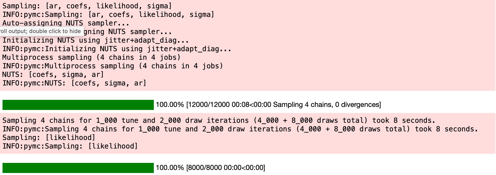
idata_arプレート表示とモデル構造をチェックしましよう。そして収束の診断を検査しましょう。
az.plot_trace(idata_ar, figsize=(10, 6), kind="rank_vlines");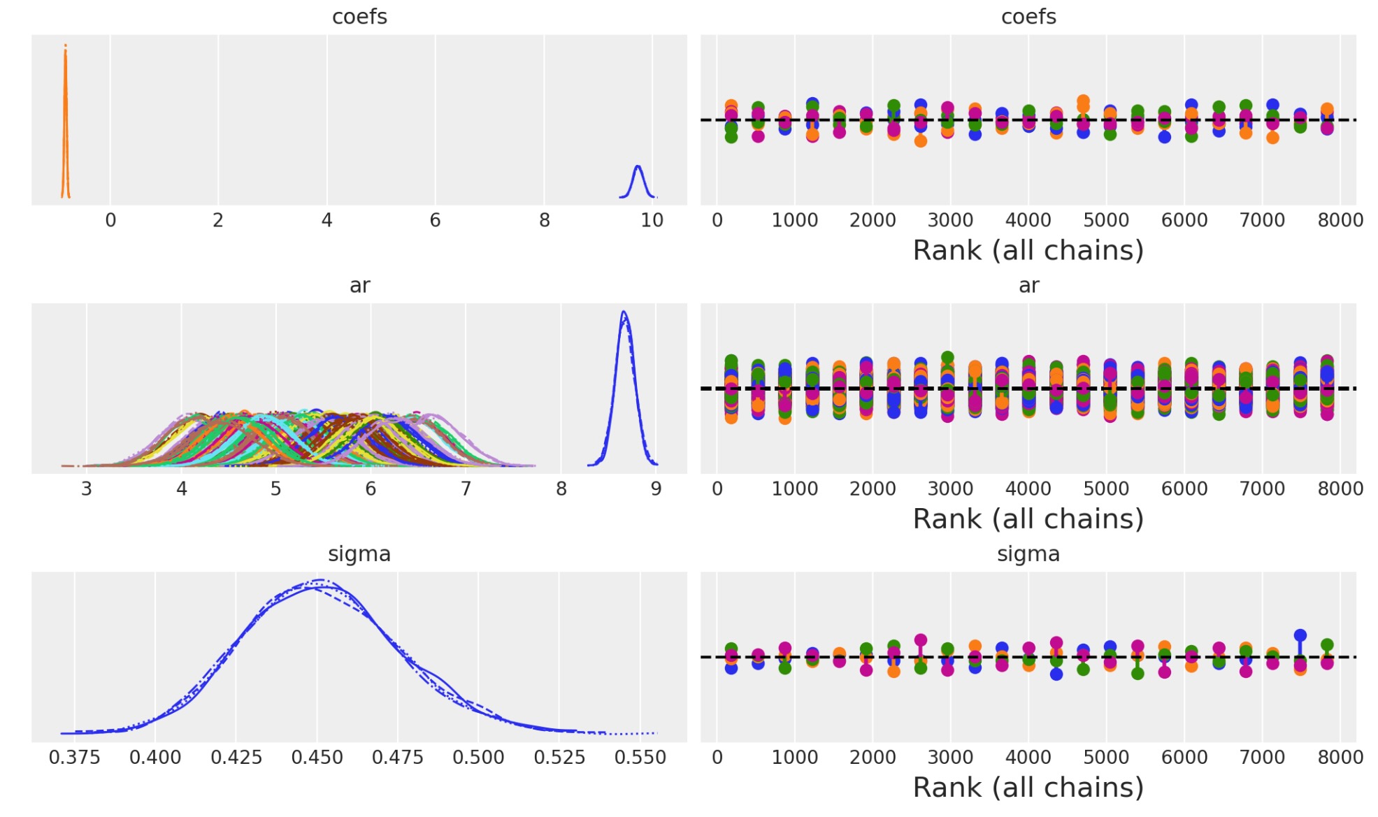
次にAR係数とシグマの終端のために結果を見積もります。
az.summary(idata_ar, var_names=["~ar"])| mean | sd | hdi_3% | hdi_97% | mcse_mean | mcse_sd | ess_bulk | ess_tail | r_hat | |
|---|---|---|---|---|---|---|---|---|---|
| coefs[0] | 9.739 | 0.093 | 9.565 | 9.911 | 0.001 | 0.001 | 12012.0 | 5877.0 | 1.0 |
| coefs[1] | -0.819 | 0.021 | -0.858 | -0.781 | 0.000 | 0.000 | 8284.0 | 6187.0 | 1.0 |
| sigma | 0.452 | 0.025 | 0.406 | 0.499 | 0.000 | 0.000 | 3038.0 | 5043.0 | 1.0 |
fig, ax = plt.subplots(figsize=(10, 4))
idata_ar.posterior.ar.mean(["chain", "draw"]).plot(ax=ax, label="Posterior Mean AR level")
ax.plot(ar1_data, "o", color="black", markersize=2, label="Observed Data")
ax.legend()
ax.set_title("Fitted AR process\nand observed data");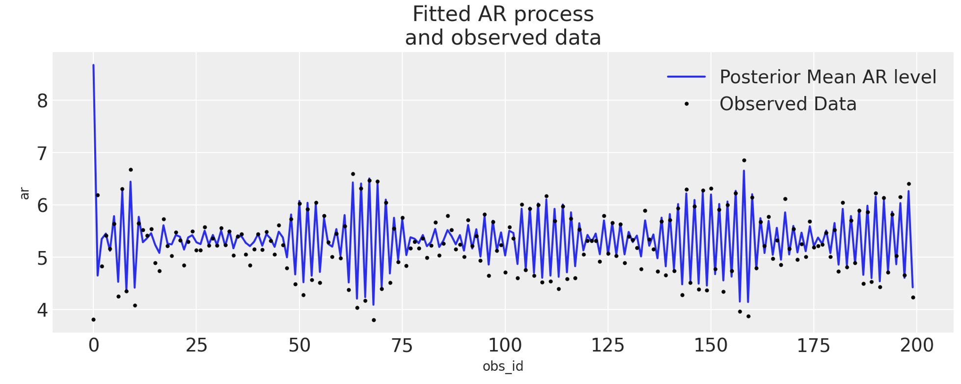
予測段階
次の段階は、GLMモデルの新しいデータのために生成する事後よく観測値から、幾分異なった働きをします。私たちは構造上のパラメータの学習後の事後分布から予測するので、学習パラメータを訓練する必要があります。別の方法では、我々が単に適合させたいモデルに帰属させたい(何らかの基礎からそれらの値を帰属させるまでの、)予測ステップの数をモデルに教えなければなりません。
具体的な形を取り扱うために、モデルに予測のための新しいデータを提供しなければなりません。そして、AR過程の学習パラメータを組み入れる方法の詳細を規定します。そうすることで、将来のために新しいAR過程を初期化します。そして、それを私たちがモデルをデータに適合させるときに学習した初期値のセットに提供します。これを実行するために、初期AR値を学習ずみ事後パラメータの周辺に非常にきつく制限するために、利用できる限り正確に、ディラック分布を使います。
prediction_length = 250
n = prediction_length - ar1_data.shape[0]
obs = list(range(prediction_length))
with AR:
    ## We need to have coords for the observations minus the lagged term to correctly centre the prediction step
    AR.add_coords({"obs_id_fut_1": range(ar1_data.shape[0] - 1, 250, 1)})
    AR.add_coords({"obs_id_fut": range(ar1_data.shape[0], 250, 1)})
    # condition on the learned values of the AR process
    # initialise the future AR process precisely at the last observed value in the AR process
    # using the special feature of the dirac delta distribution to be 0 everywhere else.
    ar1_fut = pm.AR(
        "ar1_fut",
        init_dist=pm.DiracDelta.dist(ar1[..., -1]),
        rho=coefs,
        sigma=sigma,
        constant=True,
        dims="obs_id_fut_1",
    )
    yhat_fut = pm.Normal("yhat_fut", mu=ar1_fut[1:], sigma=sigma, dims="obs_id_fut")
    # use the updated values and predict outcomes and probabilities:
    idata_preds = pm.sample_posterior_predictive(
        idata_ar, var_names=["likelihood", "yhat_fut"], predictions=True, random_seed=100
    )
自己回帰予測の条件的性質、観測データに依存している方法を理解することは重要です。私たちの2ステップでは、モデルは適合し、私たちがAR過程のパラメータのために事後分布を学習した過程を予測します。そしてそれらのパラメータを私たちの予測の中心に使います
pm.model_to_graphviz(AR)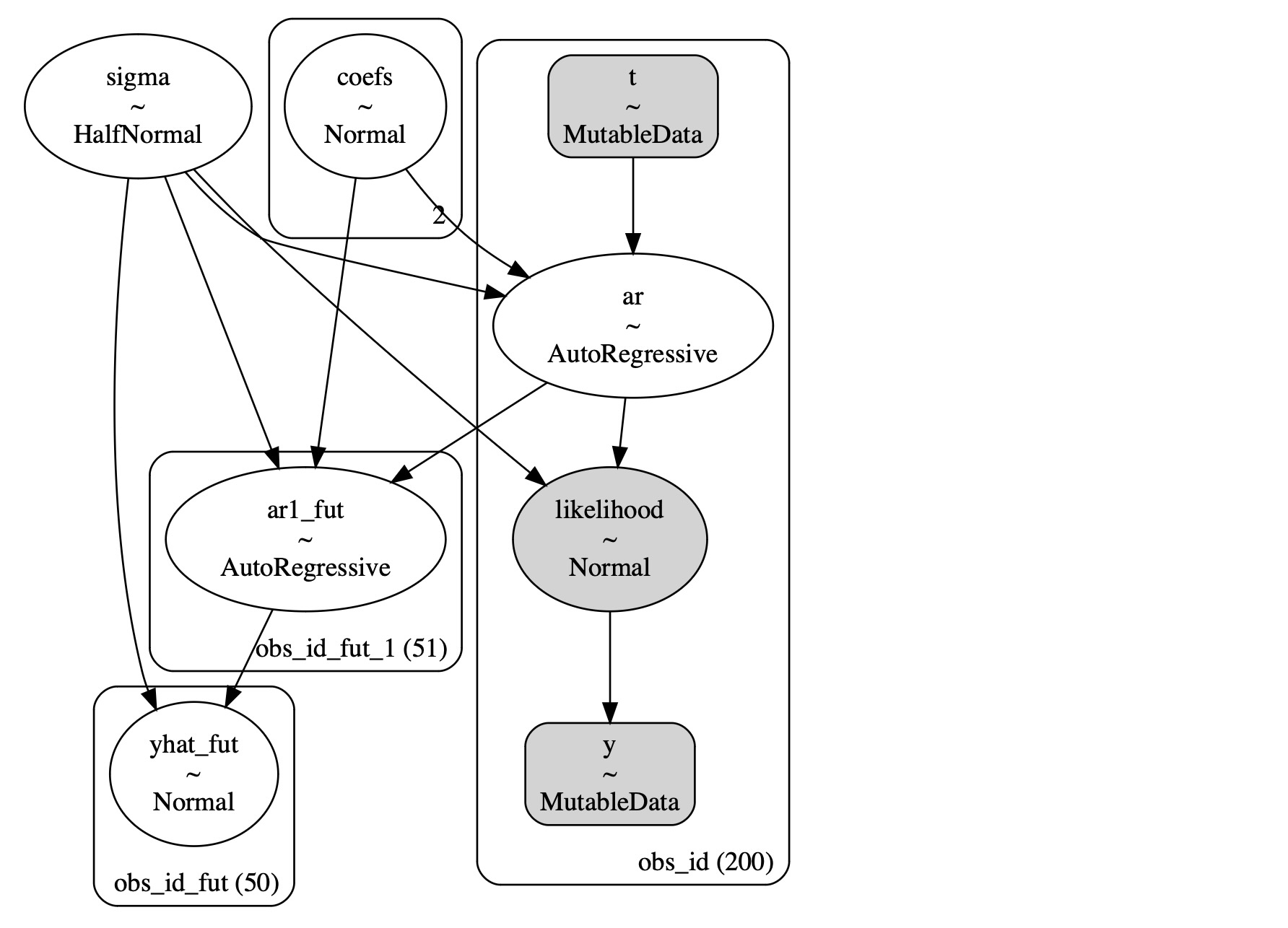
idata_predsモデルの適合と予測の調査
私たちは標準の事後予測適合に注目することができます。しかし、私たちのデータは時系列データなので、どのように事後予測分布からの出力が時間上で変化するかにも注目しなければなりません。
def plot_fits(idata_ar, idata_preds):
    palette = "plasma"
    cmap = plt.get_cmap(palette)
    percs = np.linspace(51, 99, 100)
    colors = (percs - np.min(percs)) / (np.max(percs) - np.min(percs))
    mosaic = """AABB
                CCCC"""
    fig, axs = plt.subplot_mosaic(mosaic, sharex=False, figsize=(20, 10))
    axs = [axs[k] for k in axs.keys()]
    for i, p in enumerate(percs[::-1]):
        upper = np.percentile(
            az.extract_dataset(idata_ar, group="prior_predictive", num_samples=1000)["likelihood"],
            p,
            axis=1,
        )
        lower = np.percentile(
            az.extract_dataset(idata_ar, group="prior_predictive", num_samples=1000)["likelihood"],
            100 - p,
            axis=1,
        )
        color_val = colors[i]
        axs[0].fill_between(
            x=idata_ar["constant_data"]["t"],
            y1=upper.flatten(),
            y2=lower.flatten(),
            color=cmap(color_val),
            alpha=0.1,
        )

    axs[0].plot(
        az.extract_dataset(idata_ar, group="prior_predictive", num_samples=1000)["likelihood"].mean(
            axis=1
        ),
        color="cyan",
        label="Prior Predicted Mean Realisation",
    )

    axs[0].scatter(
        x=idata_ar["constant_data"]["t"],
        y=idata_ar["constant_data"]["y"],
        color="k",
        label="Observed Data points",
    )
    axs[0].set_title("Prior Predictive Fit", fontsize=20)
    axs[0].legend()

    for i, p in enumerate(percs[::-1]):
        upper = np.percentile(
            az.extract_dataset(idata_preds, group="predictions", num_samples=1000)["likelihood"],
            p,
            axis=1,
        )
        lower = np.percentile(
            az.extract_dataset(idata_preds, group="predictions", num_samples=1000)["likelihood"],
            100 - p,
            axis=1,
        )
        color_val = colors[i]
        axs[2].fill_between(
            x=idata_preds["predictions_constant_data"]["t"],
            y1=upper.flatten(),
            y2=lower.flatten(),
            color=cmap(color_val),
            alpha=0.1,
        )

        upper = np.percentile(
            az.extract_dataset(idata_preds, group="predictions", num_samples=1000)["yhat_fut"],
            p,
            axis=1,
        )
        lower = np.percentile(
            az.extract_dataset(idata_preds, group="predictions", num_samples=1000)["yhat_fut"],
            100 - p,
            axis=1,
        )
        color_val = colors[i]
        axs[2].fill_between(
            x=idata_preds["predictions"].coords["obs_id_fut"].data,
            y1=upper.flatten(),
            y2=lower.flatten(),
            color=cmap(color_val),
            alpha=0.1,
        )

    axs[2].plot(
        az.extract_dataset(idata_preds, group="predictions", num_samples=1000)["likelihood"].mean(
            axis=1
        ),
        color="cyan",
    )
    idata_preds.predictions.yhat_fut.mean(["chain", "draw"]).plot(
        ax=axs[2], color="cyan", label="Predicted Mean Realisation"
    )
    axs[2].scatter(
        x=idata_ar["constant_data"]["t"],
        y=idata_ar["constant_data"]["y"],
        color="k",
        label="Observed Data",
    )
    axs[2].set_title("Posterior Predictions Plotted", fontsize=20)
    axs[2].axvline(np.max(idata_ar["constant_data"]["t"]), color="black")
    axs[2].legend()
    axs[2].set_xlabel("Time in Days")
    axs[0].set_xlabel("Time in Days")
    az.plot_ppc(idata_ar, ax=axs[1])


plot_fits(idata_ar, idata_preds)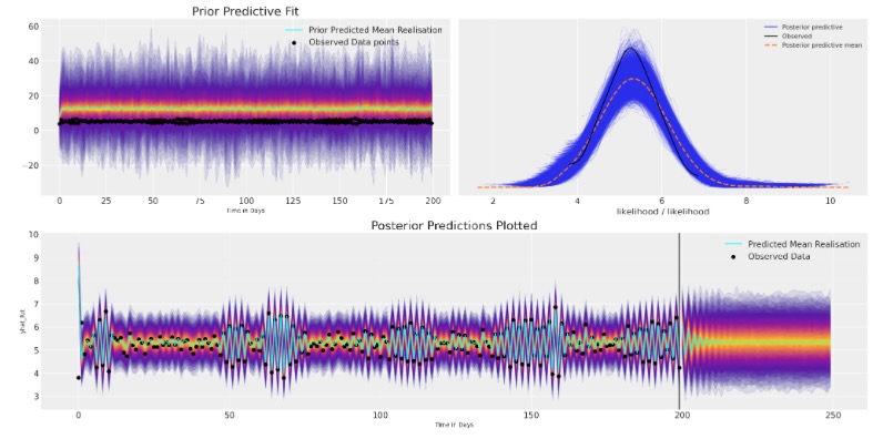
ここにモデルは収束するけれども、将来の値のために最もらしい見通しで、既存のデータに適切に適合して終了します。しかし、事前の仕様を、自己回帰関数のある種複雑な論理のせいで、値の範囲を驚くほど広範に取れるように、とても簡単に設定しました。この理由で 事前予測チェックに合うようにあなたのモデルを仕立てて、調査できるためには重要です。
2番目に平均予測が任意の長い持続的な構造を取り込みに失敗し、急速に安定したベースラインに落ち着きます。この種の短命な予測を説明するために、モデルにもっと構造を追加することができます。しかし、最初に複雑な絵を描きましょう。
複雑な絵
しばしば私たちのデータは、一つ以上の潜在的な過程を含んでいます。そして、結果を駆動する複雑な因子を持っているかもしれません。そうした複雑さを見るために、私たちのデータにトレンドを追加しましょう。私たちの予測にもっと構造を追加することによって、私たちが正確なパターンを予期し、将来のデータの出力がとどまるためのトレンドをモデルに教えます。どの構造を追加するかの選択は、モデル設計者の判断の自由になります。ー ここに簡単な例を示します。
y_t = -0.3 + np.arange(200) * -0.2 + np.random.normal(0, 10, 200)
y_t = y_t + ar1_data

fig, ax = plt.subplots(figsize=(10, 4))
ax.plot(y_t)
ax.set_title("AR Process + Trend data");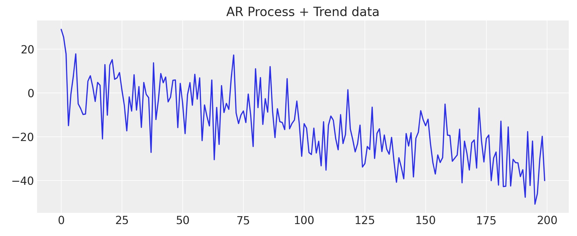
モデルを関数で覆う
def make_latent_AR_model(ar_data, priors, prediction_steps=250, full_sample=True, samples=2000):
    with pm.Model() as AR:
        pass

    t_data = list(range(len(ar_data)))
    AR.add_coord("obs_id", t_data, mutable=True)

    with AR:
        ## Data containers to enable prediction
        t = pm.MutableData("t", t_data, dims="obs_id")
        y = pm.MutableData("y", ar_data, dims="obs_id")
        # The first coefficient will be the intercept term
        coefs = pm.Normal("coefs", priors["coefs"]["mu"], priors["coefs"]["sigma"])
        sigma = pm.HalfNormal("sigma", priors["sigma"])
        # We need one init variable for each lag, hence size is variable too
        init = pm.Normal.dist(
            priors["init"]["mu"], priors["init"]["sigma"], size=priors["init"]["size"]
        )
        # Steps of the AR model minus the lags required given specification
        ar1 = pm.AR(
            "ar",
            coefs,
            sigma=sigma,
            init_dist=init,
            constant=True,
            steps=t.shape[0] - (priors["coefs"]["size"] - 1),
            dims="obs_id",
        )

        # The Likelihood
        outcome = pm.Normal("likelihood", mu=ar1, sigma=sigma, observed=y, dims="obs_id")
        ## Sampling
        idata_ar = pm.sample_prior_predictive()
        if full_sample:
            idata_ar.extend(pm.sample(samples, random_seed=100, target_accept=0.95))
            idata_ar.extend(pm.sample_posterior_predictive(idata_ar))
        else:
            return idata_ar

    n = prediction_steps - ar_data.shape[0]

    with AR:
        AR.add_coords({"obs_id_fut_1": range(ar1_data.shape[0] - 1, 250, 1)})
        AR.add_coords({"obs_id_fut": range(ar1_data.shape[0], 250, 1)})
        # condition on the learned values of the AR process
        # initialise the future AR process precisely at the last observed value in the AR process
        # using the special feature of the dirac delta distribution to be 0 probability everywhere else.
        ar1_fut = pm.AR(
            "ar1_fut",
            init_dist=pm.DiracDelta.dist(ar1[..., -1]),
            rho=coefs,
            sigma=sigma,
            constant=True,
            dims="obs_id_fut_1",
        )
        yhat_fut = pm.Normal("yhat_fut", mu=ar1_fut[1:], sigma=sigma, dims="obs_id_fut")
        # use the updated values and predict outcomes and probabilities:
        idata_preds = pm.sample_posterior_predictive(
            idata_ar, var_names=["likelihood", "yhat_fut"], predictions=True, random_seed=100
        )

    return idata_ar, idata_preds, AR
次に、仮に事前に特徴づけたモデルから将来のサンプルを撮った場合、如何に事前予測分布が、私たちの結果の暗黙の分布に影響するかを表示させるために事前仕様の数、表示を繰り返します。
priors_0 = {
    "coefs": {"mu": [-4, 0.2], "sigma": 0.1, "size": 2},
    "sigma": 8,
    "init": {"mu": 9, "sigma": 0.1, "size": 1},
}

priors_1 = {
    "coefs": {"mu": [-2, 0.2], "sigma": 0.1, "size": 2},
    "sigma": 12,
    "init": {"mu": 8, "sigma": 0.1, "size": 1},
}

priors_2 = {
    "coefs": {"mu": [0, 0.2], "sigma": 0.1, "size": 2},
    "sigma": 15,
    "init": {"mu": 8, "sigma": 0.1, "size": 1},
}

models = {}
for i, p in enumerate([priors_0, priors_1, priors_2]):
    models[i] = {}
    idata = make_latent_AR_model(y_t, p, full_sample=False)
    models[i]["idata"] = idata
fig, axs = plt.subplots(1, 3, figsize=(10, 4), sharey=True)
axs = axs.flatten()
for i, p in zip(range(3), [priors_0, priors_1, priors_2]):
    axs[i].plot(
        az.extract_dataset(models[i]["idata"], group="prior_predictive", num_samples=100)[
            "likelihood"
        ],
        color="blue",
        alpha=0.1,
    )
    axs[i].plot(y_t, "o", color="black", markersize=2)
    axs[i].set_title(
        "$y_{t+1}$" + f'= N({p["coefs"]["mu"][0]} + {p["coefs"]["mu"][1]}y$_t$, {p["sigma"]})'
    )
plt.suptitle("Prior Predictive Specifications", fontsize=20);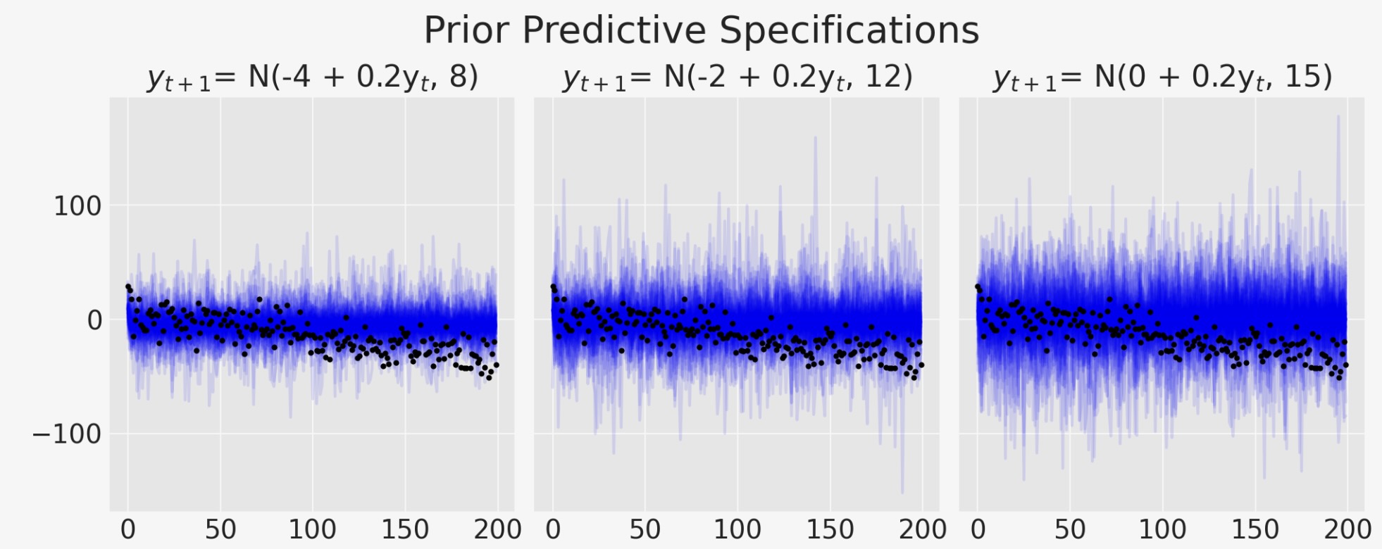
モデルがトレンドラインを取り込もうと奮闘する方法を見ることができます。モデルの変異性の増加は、データ内にある私たちが知っている方向パターンを取り込めなくなります。
priors_0 = {
    "coefs": {"mu": [-4, 0.2], "sigma": [0.5, 0.03], "size": 2},
    "sigma": 8,
    "init": {"mu": -4, "sigma": 0.1, "size": 1},
}

idata_no_trend, preds_no_trend, model = make_latent_AR_model(y_t, priors_0)
plot_fits(idata_no_trend, preds_no_trend)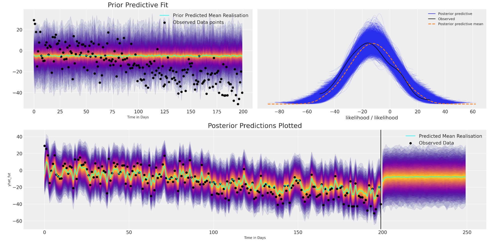
このモデルの予測はやや改善の見込みがありません。なぜなら、モデルは観察データにうまく適合するけれども、データ内の構造上のトレンドを取り込むのに完全に失敗します。そのためどのような構造的な制限もなしに、この簡単なARモデルで予測を探索するとき、非常に急速に平均値の水準の予測値に戻ります。
トレンドモデルを詳細を規定する
私たちは、データのトレンドを説明するためにモデルを定義します。そして自己回帰成分の追加モデルにこのトレンドを組み合わせます。再度、モデルが以前と同様に、しかし今度は追加の潜在的特徴を付加します。簡単な追加の組み合わせを合体させることですが、仮に私たちのモデルに最適であれば、ここではより想像的にできます。
def make_latent_AR_trend_model(
    ar_data, priors, prediction_steps=250, full_sample=True, samples=2000
):
    with pm.Model() as AR:
        pass

    t_data = list(range(len(ar_data)))
    AR.add_coord("obs_id", t_data, mutable=True)

    with AR:
        ## Data containers to enable prediction
        t = pm.MutableData("t", t_data, dims="obs_id")
        y = pm.MutableData("y", ar_data, dims="obs_id")
        # The first coefficient will be the intercept term
        coefs = pm.Normal("coefs", priors["coefs"]["mu"], priors["coefs"]["sigma"])
        sigma = pm.HalfNormal("sigma", priors["sigma"])
        # We need one init variable for each lag, hence size is variable too
        init = pm.Normal.dist(
            priors["init"]["mu"], priors["init"]["sigma"], size=priors["init"]["size"]
        )
        # Steps of the AR model minus the lags required given specification
        ar1 = pm.AR(
            "ar",
            coefs,
            sigma=sigma,
            init_dist=init,
            constant=True,
            steps=t.shape[0] - (priors["coefs"]["size"] - 1),
            dims="obs_id",
        )

        ## Priors for the linear trend component
        alpha = pm.Normal("alpha", priors["alpha"]["mu"], priors["alpha"]["sigma"])
        beta = pm.Normal("beta", priors["beta"]["mu"], priors["beta"]["sigma"])
        trend = pm.Deterministic("trend", alpha + beta * t, dims="obs_id")

        mu = ar1 + trend

        # The Likelihood
        outcome = pm.Normal("likelihood", mu=mu, sigma=sigma, observed=y, dims="obs_id")
        ## Sampling
        idata_ar = pm.sample_prior_predictive()
        if full_sample:
            idata_ar.extend(pm.sample(samples, random_seed=100, target_accept=0.95))
            idata_ar.extend(pm.sample_posterior_predictive(idata_ar))
        else:
            return idata_ar

    n = prediction_steps - ar_data.shape[0]

    with AR:
        AR.add_coords({"obs_id_fut_1": range(ar1_data.shape[0] - 1, prediction_steps, 1)})
        AR.add_coords({"obs_id_fut": range(ar1_data.shape[0], prediction_steps, 1)})
        t_fut = pm.MutableData("t_fut", list(range(ar1_data.shape[0], prediction_steps, 1)))
        # condition on the learned values of the AR process
        # initialise the future AR process precisely at the last observed value in the AR process
        # using the special feature of the dirac delta distribution to be 0 probability everywhere else.
        ar1_fut = pm.AR(
            "ar1_fut",
            init_dist=pm.DiracDelta.dist(ar1[..., -1]),
            rho=coefs,
            sigma=sigma,
            constant=True,
            dims="obs_id_fut_1",
        )
        trend = pm.Deterministic("trend_fut", alpha + beta * t_fut, dims="obs_id_fut")
        mu = ar1_fut[1:] + trend

        yhat_fut = pm.Normal("yhat_fut", mu=mu, sigma=sigma, dims="obs_id_fut")
        # use the updated values and predict outcomes and probabilities:
        idata_preds = pm.sample_posterior_predictive(
            idata_ar, var_names=["likelihood", "yhat_fut"], predictions=True, random_seed=100
        )

    return idata_ar, idata_preds, AR
私たちは、負のトレンドとデータ推移の方向を反映した標準偏差の範囲の事前の特等付けによって、このモデルを適合させます。
priors_0 = {
    "coefs": {"mu": [0.2, 0.2], "sigma": [0.5, 0.03], "size": 2},
    "alpha": {"mu": -4, "sigma": 0.1},
    "beta": {"mu": -0.1, "sigma": 0.2},
    "sigma": 8,
    "init": {"mu": -4, "sigma": 0.1, "size": 1},
}


idata_trend, preds_trend, model = make_latent_AR_trend_model(y_t, priors_0, full_sample=True)
pm.model_to_graphviz(model)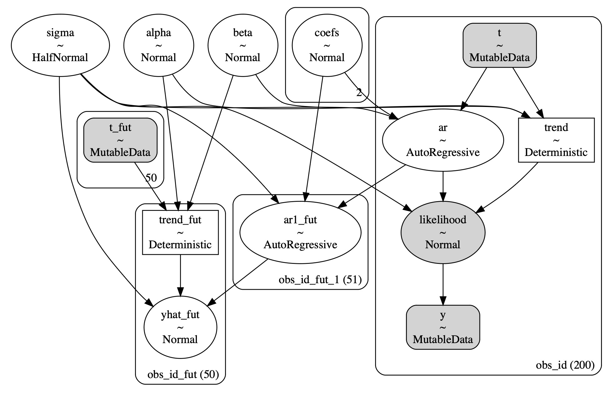
私たちは、プレートの表示でより明快な構造を見ることができます。そして、この追加構造は、時系列データのトレンドの方向の適切な適合に寄与します。
plot_fits(idata_trend, preds_trend);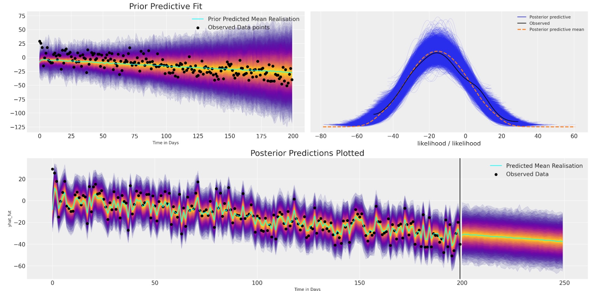
az.summary(idata_trend, var_names=["coefs", "sigma", "alpha", "beta"])| mean | sd | hdi_3% | hdi_97% | mcse_mean | mcse_sd | ess_bulk | ess_tail | r_hat | |
|---|---|---|---|---|---|---|---|---|---|
| coefs[0] | 0.977 | 0.482 | 0.089 | 1.893 | 0.009 | 0.006 | 2866.0 | 4677.0 | 1.0 |
| coefs[1] | 0.204 | 0.030 | 0.150 | 0.259 | 0.000 | 0.000 | 8115.0 | 6438.0 | 1.0 |
| sigma | 8.172 | 0.420 | 7.414 | 8.982 | 0.008 | 0.006 | 2870.0 | 4201.0 | 1.0 |
| alpha | -3.971 | 0.101 | -4.164 | -3.783 | 0.001 | 0.001 | 9192.0 | 5998.0 | 1.0 |
| beta | -0.140 | 0.009 | -0.157 | -0.122 | 0.000 | 0.000 | 1776.0 | 3211.0 | 1.0 |
さらに進んだ複雑な状況
次に、データに季節成分を追加します。ベイズ構造上の時系列モデルのデータのこの様相を、どのように回復することができるか見ていきます。再度、これが、現実に私たちのデータがしばしば、多重に収束する影響の結果の理由です。これらの影響は、各成分に適切な重みを割り当てることで私たちの推測モデルが確認する、追加のベイズ構造上のモデルで取り込むことができます。
t_data = list(range(200))
n_order = 10
periods = np.array(t_data) / 7

fourier_features = pd.DataFrame(
    {
        f"{func}_order_{order}": getattr(np, func)(2 * np.pi * periods * order)
        for order in range(1, n_order + 1)
        for func in ("sin", "cos")
    }
)

y_t_s = y_t + 20 * fourier_features["sin_order_1"]

fig, ax = plt.subplots(figsize=(10, 4))
ax.plot(y_t_s)
ax.set_title("AR + Trend + Seasonality");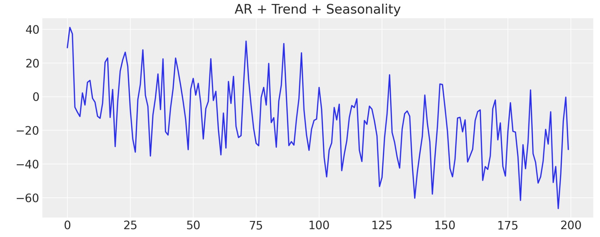
このモデルを適合する鍵は、季節の影響を説明するのに役立つ合成フーリエ特徴を通すことを理解することです。これは稼働します。なぜなら、(大雑把に言って)複雑な振動現象を、正弦波とコサイン波の重みづけた組み合わせを使うことで、適合するように試みます。そのため私たちは、他の任意の特徴をもつ変数を回帰モデルに追加するように、これらの正弦波とコサイン波を追加します。
しかし、重みづけた集計を使うことにより、モデルが、予測段階でもなお、それらの合成の特徴の線形の組み合わせを予期します。そのようにして、将来の出力であっても、それらの特徴を提供することができます。この事実は、私たちが追加を必要とするかもしれない、週の曜日、休日のダミー変数、またはその他の任意の他の種類の予測に使う特徴の鍵のままです。仮に特徴が観察データに適合することが必要とされるならば、その特徴は予測段階でも利用できるに違いありません。
トレンド+季節要因モデルの詳細規定
def make_latent_AR_trend_seasonal_model(
    ar_data, ff, priors, prediction_steps=250, full_sample=True, samples=2000
):
    with pm.Model() as AR:
        pass

    ff = ff.to_numpy().T
    t_data = list(range(len(ar_data)))
    AR.add_coord("obs_id", t_data, mutable=True)
    ## The fourier features must be mutable to allow for addition fourier features to be
    ## passed in the prediction step.
    AR.add_coord("fourier_features", np.arange(len(ff)), mutable=True)

    with AR:
        ## Data containers to enable prediction
        t = pm.MutableData("t", t_data, dims="obs_id")
        y = pm.MutableData("y", ar_data, dims="obs_id")
        # The first coefficient will be the intercept term
        coefs = pm.Normal("coefs", priors["coefs"]["mu"], priors["coefs"]["sigma"])
        sigma = pm.HalfNormal("sigma", priors["sigma"])
        # We need one init variable for each lag, hence size is variable too
        init = pm.Normal.dist(
            priors["init"]["mu"], priors["init"]["sigma"], size=priors["init"]["size"]
        )
        # Steps of the AR model minus the lags required given specification
        ar1 = pm.AR(
            "ar",
            coefs,
            sigma=sigma,
            init_dist=init,
            constant=True,
            steps=t.shape[0] - (priors["coefs"]["size"] - 1),
            dims="obs_id",
        )

        ## Priors for the linear trend component
        alpha = pm.Normal("alpha", priors["alpha"]["mu"], priors["alpha"]["sigma"])
        beta = pm.Normal("beta", priors["beta"]["mu"], priors["beta"]["sigma"])
        trend = pm.Deterministic("trend", alpha + beta * t, dims="obs_id")

        ## Priors for seasonality
        beta_fourier = pm.Normal(
            "beta_fourier",
            mu=priors["beta_fourier"]["mu"],
            sigma=priors["beta_fourier"]["sigma"],
            dims="fourier_features",
        )
        fourier_terms = pm.MutableData("fourier_terms", ff)
        seasonality = pm.Deterministic(
            "seasonality", pm.math.dot(beta_fourier, fourier_terms), dims="obs_id"
        )

        mu = ar1 + trend + seasonality

        # The Likelihood
        outcome = pm.Normal("likelihood", mu=mu, sigma=sigma, observed=y, dims="obs_id")
        ## Sampling
        idata_ar = pm.sample_prior_predictive()
        if full_sample:
            idata_ar.extend(pm.sample(samples, random_seed=100, target_accept=0.95))
            idata_ar.extend(pm.sample_posterior_predictive(idata_ar))
        else:
            return idata_ar

    n = prediction_steps - ar_data.shape[0]
    n_order = 10
    periods = (ar_data.shape[0] + np.arange(n)) / 7

    fourier_features_new = pd.DataFrame(
        {
            f"{func}_order_{order}": getattr(np, func)(2 * np.pi * periods * order)
            for order in range(1, n_order + 1)
            for func in ("sin", "cos")
        }
    )

    with AR:
        AR.add_coords({"obs_id_fut_1": range(ar1_data.shape[0] - 1, prediction_steps, 1)})
        AR.add_coords({"obs_id_fut": range(ar1_data.shape[0], prediction_steps, 1)})
        t_fut = pm.MutableData(
            "t_fut", list(range(ar1_data.shape[0], prediction_steps, 1)), dims="obs_id_fut"
        )
        ff_fut = pm.MutableData("ff_fut", fourier_features_new.to_numpy().T)
        # condition on the learned values of the AR process
        # initialise the future AR process precisely at the last observed value in the AR process
        # using the special feature of the dirac delta distribution to be 0 probability everywhere else.
        ar1_fut = pm.AR(
            "ar1_fut",
            init_dist=pm.DiracDelta.dist(ar1[..., -1]),
            rho=coefs,
            sigma=sigma,
            constant=True,
            dims="obs_id_fut_1",
        )
        trend = pm.Deterministic("trend_fut", alpha + beta * t_fut, dims="obs_id_fut")
        seasonality = pm.Deterministic(
            "seasonality_fut", pm.math.dot(beta_fourier, ff_fut), dims="obs_id_fut"
        )
        mu = ar1_fut[1:] + trend + seasonality

        yhat_fut = pm.Normal("yhat_fut", mu=mu, sigma=sigma, dims="obs_id_fut")
        # use the updated values and predict outcomes and probabilities:
        idata_preds = pm.sample_posterior_predictive(
            idata_ar, var_names=["likelihood", "yhat_fut"], predictions=True, random_seed=743
        )

    return idata_ar, idata_preds, AR
priors_0 = {
"coefs": {"mu": [0.2, 0.2], "sigma": [0.5, 0.03], "size": 2},
"alpha": {"mu": -4, "sigma": 0.1},
"beta": {"mu": -0.1, "sigma": 0.2},
"beta_fourier": {"mu": 0, "sigma": 2},
"sigma": 8,
"init": {"mu": -4, "sigma": 0.1, "size": 1},
}
idata_t_s, preds_t_s, model = make_latent_AR_trend_seasonal_model(y_t_s, fourier_features, priors_0)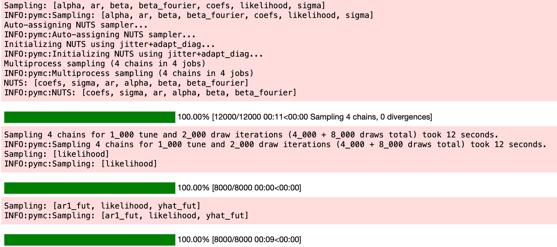
pm.model_to_graphviz(model)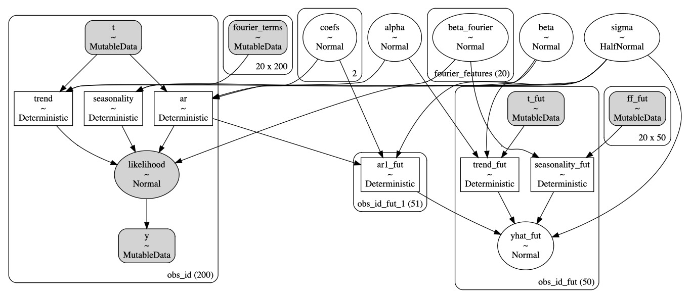
az.summary(idata_t_s, var_names=["alpha", "beta", "coefs", "beta_fourier"])| mean | sd | hdi_3% | hdi_97% | mcse_mean | mcse_sd | ess_bulk | ess_tail | r_hat | |
|---|---|---|---|---|---|---|---|---|---|
| alpha | -3.985 | 0.099 | -4.171 | -3.798 | 0.001 | 0.001 | 16249.0 | 6174.0 | 1.0 |
| beta | -0.180 | 0.013 | -0.204 | -0.156 | 0.000 | 0.000 | 3372.0 | 4549.0 | 1.0 |
| coefs[0] | 0.498 | 0.484 | -0.397 | 1.445 | 0.008 | 0.006 | 3658.0 | 5490.0 | 1.0 |
| coefs[1] | 0.192 | 0.030 | 0.139 | 0.250 | 0.000 | 0.000 | 11149.0 | 5637.0 | 1.0 |
| beta_fourier[0] | 5.896 | 1.646 | 2.830 | 8.891 | 0.018 | 0.013 | 8527.0 | 6306.0 | 1.0 |
| beta_fourier[1] | 0.216 | 1.674 | -2.833 | 3.446 | 0.017 | 0.018 | 9184.0 | 5691.0 | 1.0 |
| beta_fourier[2] | -0.025 | 1.626 | -3.231 | 2.852 | 0.017 | 0.018 | 9174.0 | 5939.0 | 1.0 |
| beta_fourier[3] | 0.219 | 1.644 | -2.865 | 3.314 | 0.017 | 0.017 | 9017.0 | 6496.0 | 1.0 |
| beta_fourier[4] | -0.078 | 1.640 | -3.065 | 3.028 | 0.018 | 0.017 | 8620.0 | 6288.0 | 1.0 |
| beta_fourier[5] | -0.261 | 1.711 | -3.587 | 2.839 | 0.018 | 0.018 | 9111.0 | 6223.0 | 1.0 |
| beta_fourier[6] | 0.056 | 1.666 | -3.076 | 3.109 | 0.019 | 0.017 | 7752.0 | 6274.0 | 1.0 |
| beta_fourier[7] | -0.232 | 1.679 | -3.406 | 2.866 | 0.016 | 0.018 | 11024.0 | 6275.0 | 1.0 |
| beta_fourier[8] | 0.045 | 1.685 | -3.086 | 3.284 | 0.017 | 0.018 | 9883.0 | 6284.0 | 1.0 |
| beta_fourier[9] | 0.229 | 1.661 | -2.985 | 3.294 | 0.018 | 0.018 | 8564.0 | 6401.0 | 1.0 |
| beta_fourier[10] | -5.892 | 1.676 | -8.991 | -2.663 | 0.018 | 0.013 | 8887.0 | 5964.0 | 1.0 |
| beta_fourier[11] | 0.243 | 1.667 | -2.857 | 3.419 | 0.018 | 0.018 | 8277.0 | 5872.0 | 1.0 |
| beta_fourier[12] | -0.028 | 1.976 | -3.707 | 3.726 | 0.016 | 0.024 | 15172.0 | 5649.0 | 1.0 |
| beta_fourier[13] | 6.061 | 1.388 | 3.358 | 8.597 | 0.024 | 0.017 | 3456.0 | 4639.0 | 1.0 |
| beta_fourier[14] | 5.874 | 1.646 | 2.770 | 8.991 | 0.017 | 0.012 | 9603.0 | 6446.0 | 1.0 |
| beta_fourier[15] | 0.237 | 1.670 | -3.035 | 3.287 | 0.018 | 0.019 | 8840.0 | 6068.0 | 1.0 |
| beta_fourier[16] | -0.054 | 1.682 | -3.186 | 3.073 | 0.017 | 0.018 | 10017.0 | 6002.0 | 1.0 |
| beta_fourier[17] | 0.257 | 1.663 | -2.785 | 3.401 | 0.018 | 0.018 | 8829.0 | 6210.0 | 1.0 |
| beta_fourier[18] | -0.076 | 1.642 | -3.125 | 3.045 | 0.018 | 0.017 | 8584.0 | 6664.0 | 1.0 |
| beta_fourier[19] | -0.259 | 1.645 | -3.250 | 2.887 | 0.017 | 0.018 | 9233.0 | 6334.0 | 1.0 |
plot_fits(idata_t_s, preds_t_s)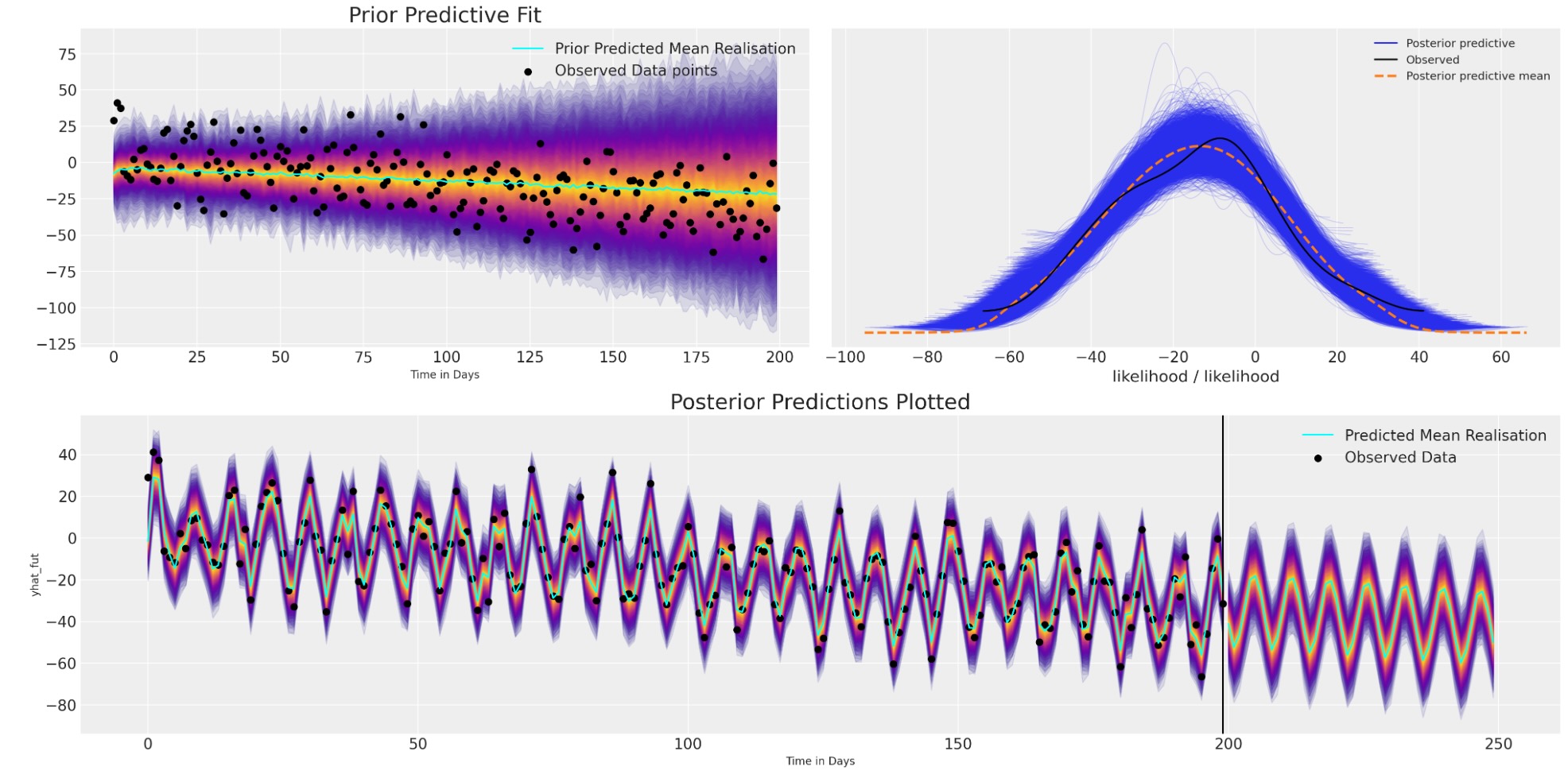
私たちはここで、どのようにモデルの適合が、再度、広範囲の構造とデータのトレンドを回復するかを見ることができます。しかし、追加で季節効果の振動とその将来の振動の推測を取り込みました。
備考
ベイジアンモデルの拡張は、柔軟性を拡大し、各モデル化のタスクを提示します。幸いにもこのノートは、あなたの使用ケースに最適であるモデルを構築するときに、考慮する価値のある多様な組み合わせの特色を提供します。予測するために如何にベイジアン構造化時系列アプローチが、私たちのデータ構造を示し、将来の構造を推測することができるか見てきました。私たちは、モデルを生成するデータに異なる仮定をコード化し、事後予測チェックにより観測データに逆らったモデルを校正する方法を見てきました。
特に、自己回帰モデル化のケースで、明確に構造上の成分の学習した事後分布を必要とします。上記の私たちが考えるこの様相はある種、純粋なベイズ学習の例です。
製作者
著作者:Nathaniel Forde 2022年10月 ’アルゴリズムの検査ブログ’(Examined Algorithm Blog) より