gp.Latentクラスは直接、近似なしでガウス過程を実装します。与えられた平均と共分散関数は、私たちは関数f(x)に事前分布を置くことができます。

"潜在”と呼ばれます、なぜなら、GPはそれ自身、潜在変数としてモデルに含んでいます。それは、gp.Marginalのケースのように境界から外れません。gp.Latentは違い、あなたがgp.MarginalでトレースのGP事後分布からサンプルを見つけなくとも良いのです。これは、主流な直接のGPの実装です。なぜなら、特別な尤度関数や、データ構造、共分散行列を仮定しません。
.priorメソッド
priorメソッドは、多変量正規事前分布をPyMCモデルに追加します。GP関数の値のベクターを覆って,f,

ここで、ベクターmx, と行列Kxxは、入力xを覆って評価された平均ベクターと共分散行列です。デフォルトでは、PyMCは事前分布を、共分散行列のコレスキー因子でそれを回転させることによって、hood下のfで再パラメータ化します。これは変換したランダム変数vの共分散行列を減少させることで、サンプリングを改良します。パラメータ化したモデルは、

再パラメータ化のより詳しい情報は、セクション 多変量分布から値を出力する を参照してください。
.conditionalメソッド
条件付きメソッドは、オリジナルデータセットの部分ではない関数の値のための予測分布を実装します。この分布は、

私たちが上で定義した同じ、gpオブジェクトを使うことで、私たちは、この分布とランダム変数を構築することができます。
# vector of new X points we want to predict the function at
X_star = np.linspace(0, 2, 100)[:, None]

with latent_gp_model:
    f_star = gp.conditional("f_star", X_star)
例1:ステユーデント-T分布のノイズの回帰
以下の例はgp.Latentクラスを使ったGP事前分布の簡単なモデルを規定する方法を示します。私たちは、データを生成するためにGPを使います。そのため、私たちは、私たちが実行した推定が正しいことを検証できます。尤度が正規でなく、ステューデント-TがIIDであることに注意してください。尤度がガウシアンの時の、より効果的な実装は、gp.Marginalを使うことです。
import arviz as az
import matplotlib.pyplot as plt
import numpy as np
import pymc as pm
%config InlineBackend.figure_format = 'retina'
RANDOM_SEED = 8998
rng = np.random.default_rng(RANDOM_SEED)
az.style.use("arviz-darkgrid")n = 50 # The number of data points
X = np.linspace(0, 10, n)[:, None] # The inputs to the GP must be arranged as a column vector
# Define the true covariance function and its parameters
ell_true = 1.0
eta_true = 4.0
cov_func = eta_true**2 * pm.gp.cov.ExpQuad(1, ell_true)
# A mean function that is zero everywhere
mean_func = pm.gp.mean.Zero()
# The latent function values are one sample from a multivariate normal
# Note that we have to call `eval()` because PyMC built on top of Theano
f_true = pm.draw(pm.MvNormal.dist(mu=mean_func(X), cov=cov_func(X)), 1, random_seed=rng)
# The observed data is the latent function plus a small amount of T distributed noise
# The standard deviation of the noise is `sigma`, and the degrees of freedom is `nu`
sigma_true = 1.0
nu_true = 5.0
y = f_true + sigma_true * rng.normal(size=n)
## Plot the data and the unobserved latent function
fig = plt.figure(figsize=(10, 4))
ax = fig.gca()
ax.plot(X, f_true, "dodgerblue", lw=3, label="True generating function 'f'")
ax.plot(X, y, "ok", ms=3, label="Observed data")
ax.set_xlabel("X")
ax.set_ylabel("y")
plt.legend(frameon=True);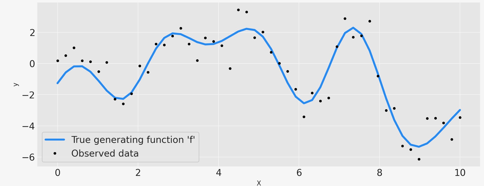
上のデータは、ノイズで汚されている未知の関数f(x),の黒い点でマークされた観測値を示しています。真の関数は青で示されてます。
PyMCでコーディングしたモデル
ここはPyMCによるモデルです。私たちは、長さのスケールのパラメータを覆う事前分布に有益なpm.Gamma()を使います。そして、週単位で有益なpm.HalfNormal()を共分散関数のスケール、ノイズのスケールの事前分布に使います。pm.Ganmma(2,0.5)事前分布は、ノイズパラメータの自由度を割り当てます。最後に、GP事前分布は、未知の関数に置かれます。ガウス過程分布の事前分布の選択のより詳しい情報は、Stan の人々によるいくつかの推薦をチェックしてください。
with pm.Model() as model:
    ell = pm.Gamma("ell", alpha=2, beta=1)
    eta = pm.HalfNormal("eta", sigma=5)

    cov = eta**2 * pm.gp.cov.ExpQuad(1, ell)
    gp = pm.gp.Latent(cov_func=cov)

    f = gp.prior("f", X=X)

    sigma = pm.HalfNormal("sigma", sigma=2.0)
    nu = 1 + pm.Gamma(
        "nu", alpha=2, beta=0.1
    )  # add one because student t is undefined for degrees of freedom less than one
    y_ = pm.StudentT("y", mu=f, lam=1.0 / sigma, nu=nu, observed=y)

    idata = pm.sample(1000, tune=1000, chains=2, cores=1)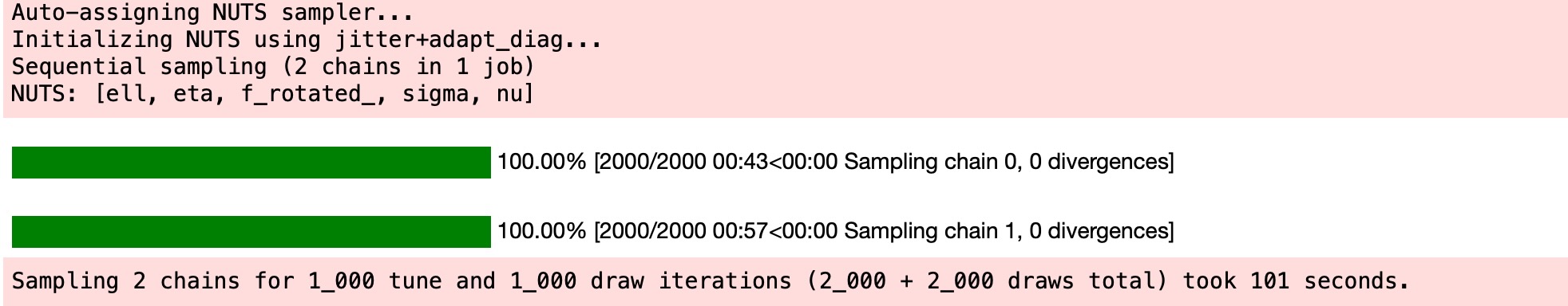
# check Rhat, values above 1 may indicate convergence issues
n_nonconverged = int(
    np.sum(az.rhat(idata)[["eta", "ell", "sigma", "f_rotated_"]].to_array() > 1.03).values
)
if n_nonconverged == 0:
    print("No Rhat values above 1.03, \N{check mark}")
else:
    print(f"The MCMC chains for {n_nonconverged} RVs appear not to have converged.")
No Rhat values above 1.03, ✓
結果
二つの共分散関数のハイパーパラメータの接合事後分布は、以下の左のパネルに図示してあります。右のパネルは、ノイズの標準偏差と尤度の自由度のパラメータの接合事後分布です。右の青線は真の値を示します。それは、通常GPからの関数で出力されます。
fig, axs = plt.subplots(1, 2, figsize=(10, 4))
axs = axs.flatten()

# plot eta vs ell
az.plot_pair(
    idata,
    var_names=["eta", "ell"],
    kind=["hexbin"],
    ax=axs[0],
    gridsize=25,
    divergences=True,
)
axs[0].axvline(x=eta_true, color="dodgerblue")
axs[0].axhline(y=ell_true, color="dodgerblue")

# plot nu vs sigma
az.plot_pair(
    idata,
    var_names=["nu", "sigma"],
    kind=["hexbin"],
    ax=axs[1],
    gridsize=25,
    divergences=True,
)

axs[1].axvline(x=nu_true, color="dodgerblue")
axs[1].axhline(y=sigma_true, color="dodgerblue");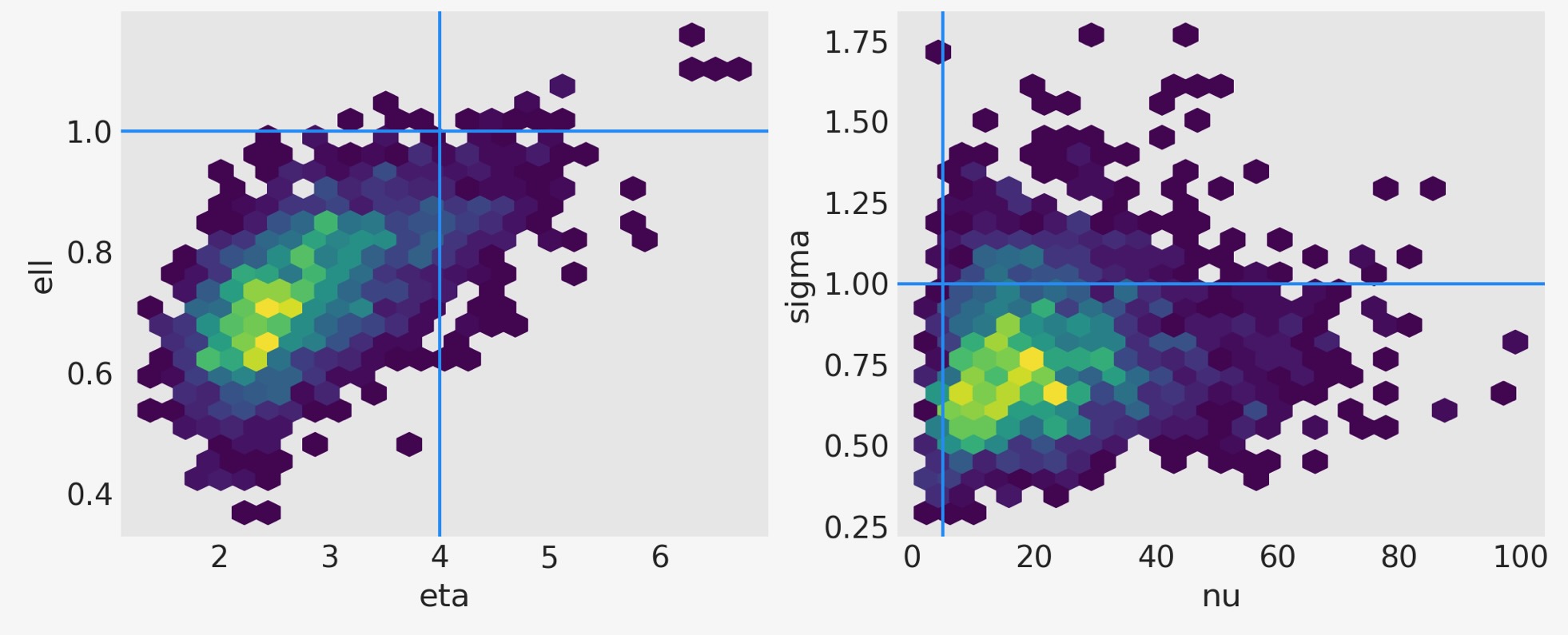
f_post = az.extract(idata, var_names="f").transpose("sample", ...)
f_post
xarray.DataArray
'f'
- sample: 2000
- f_dim_0: 50
- array([[ 0.57223296, 0.52293924, 0.25263088, ..., -4.3261952 , -4.25310038, -4.1830545 ], [ 1.06640163, 1.64173795, 1.8392588 , ..., -3.45409032, -3.7328924 , -3.89459332], [-0.07305491, 0.32960451, 0.75937892, ..., -3.11836799, -2.86881492, -3.09680561], ..., [ 0.24859838, 0.59755008, 0.71793926, ..., -3.58537587, -4.13471444, -5.00106719], [ 0.24859838, 0.59755008, 0.71793926, ..., -3.58537587, -4.13471444, -5.00106719], [ 0.52317792, 0.01741743, -0.34162981, ..., -3.51620817, -3.18992857, -3.0321463 ]])
- Coordinates:
- f_dim_0(f_dim_0)int640 1 2 3 4 5 6 ... 44 45 46 47 48 49
- sample(sample)objectMultiIndex
- chain(sample)int640 0 0 0 0 0 0 0 ... 1 1 1 1 1 1 1 1
- draw(sample)int640 1 2 3 4 5 ... 995 996 997 998 999
- Indexes: (2)
- Attributes: (0)
下は、GPの事後分布です。
# plot the results
fig = plt.figure(figsize=(10, 4))
ax = fig.gca()

# plot the samples from the gp posterior with samples and shading
from pymc.gp.util import plot_gp_dist

f_post = az.extract(idata, var_names="f").transpose("sample", ...)
plot_gp_dist(ax, f_post, X)

# plot the data and the true latent function
ax.plot(X, f_true, "dodgerblue", lw=3, label="True generating function 'f'")
ax.plot(X, y, "ok", ms=3, label="Observed data")

# axis labels and title
plt.xlabel("X")
plt.ylabel("True f(x)")
plt.title("Posterior distribution over $f(x)$ at the observed values")
plt.legend();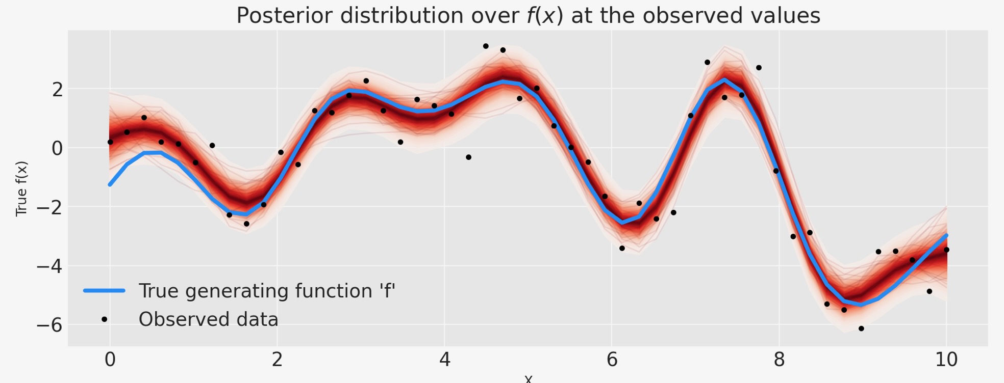
赤い編みかけで見られるのは、GP事前分布の関数を覆った事後分布は、両方の適合を表す大きな仕事であり、加法ノイズに起因した不確実性です。結果は、ステューデント-Tノイズモデルからの外れ値のせいで過度に適合しません。
conditionalを使った予測
次に、私たちは、条件付き分布を追加することで、モデルを拡張します。そのため、私たちは、新しいxの位置を予測することができます。これを実行するために、私たちは、自分ものモデルをGPのconditional分布で拡張します。その時、私たちは、トレースとsample_posterior_predictive関数を使って、それからサンプルできます。これは、Stanがその generated_qauntities{…}ブロックを、使う方法と同様のものです。私たちは、NUTSサンプリングの前に、モデルのgp.conditionalを含めることができます。しかし、これらのステップを分離した方が効果的です。
n_new = 200
X_new = np.linspace(-4, 14, n_new)[:, None]

# add the GP conditional to the model, given the new X values
with model:
    f_pred = gp.conditional("f_pred", X_new, jitter=1e-4)

# Sample from the GP conditional distribution
with model:
    ppc = pm.sample_posterior_predictive(idata.posterior, var_names=["f_pred"])
    idata.extend(ppc)
fig = plt.figure(figsize=(10, 4))
ax = fig.gca()

f_pred = az.extract(idata.posterior_predictive, var_names="f_pred").transpose("sample", ...)
plot_gp_dist(ax, f_pred, X_new)

ax.plot(X, f_true, "dodgerblue", lw=3, label="True generating function 'f'")
ax.plot(X, y, "ok", ms=3, label="Observed data")

ax.set_xlabel("X")
ax.set_ylabel("True f(x)")
ax.set_title("Conditional distribution of f_*, given f")
plt.legend();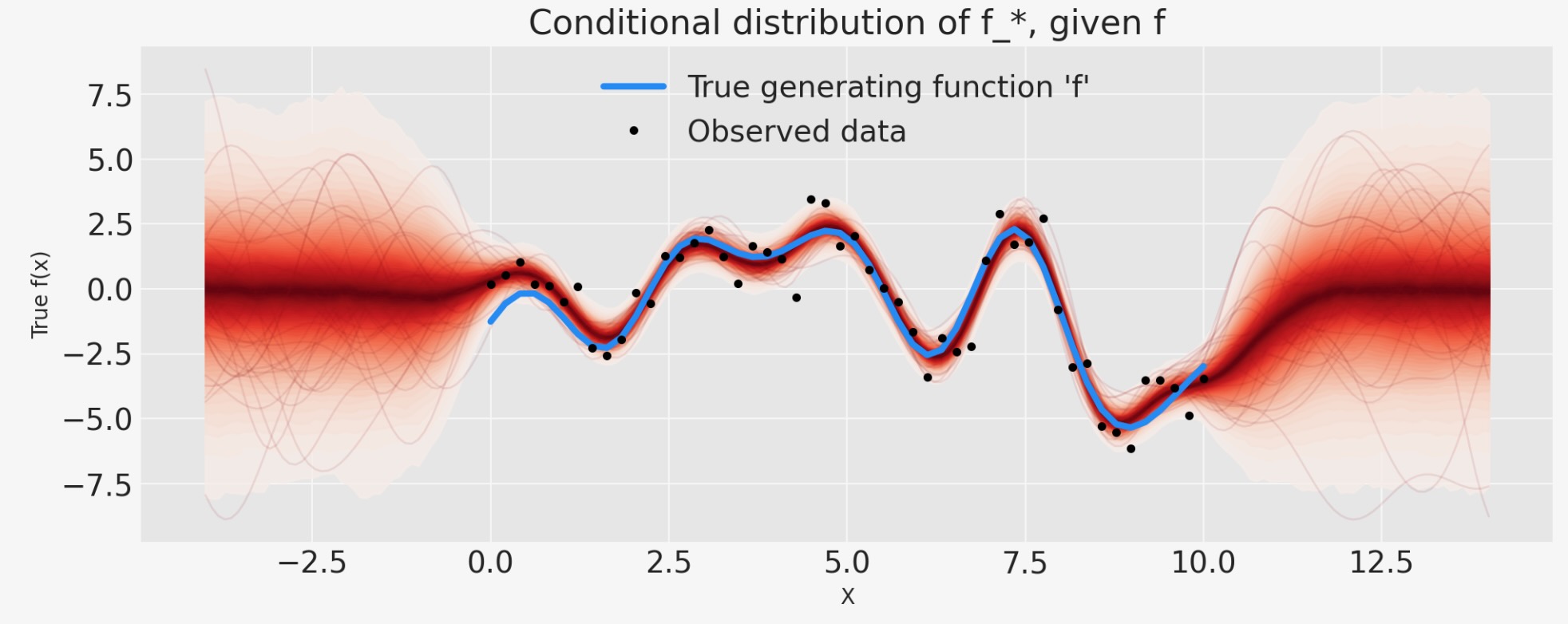
例2:分類
最初に、私たちはいくらかのデータを生成するのにGPを使います。それは、ベルヌーイ分布に従います。ここでp はある確率でゼロの代わりにxの関数になります。私は、種をリセットし、もっとフェイクデータポイントを追加します、なぜなら、モデルが少数の観測で、0.5の周りの変位に気づくのは困難になるからです。
# reset the random seed for the new example
RANDOM_SEED = 8888
rng = np.random.default_rng(RANDOM_SEED)

# number of data points
n = 300

# x locations
x = np.linspace(0, 10, n)

# true covariance
ell_true = 0.5
eta_true = 1.0
cov_func = eta_true**2 * pm.gp.cov.ExpQuad(1, ell_true)
K = cov_func(x[:, None]).eval()

# zero mean function
mean = np.zeros(n)

# sample from the gp prior
f_true = pm.draw(pm.MvNormal.dist(mu=mean, cov=K), 1, random_seed=rng)

# Sample the GP through the likelihood
y = pm.Bernoulli.dist(p=pm.math.invlogit(f_true)).eval()
fig = plt.figure(figsize=(10, 4))
ax = fig.gca()
ax.plot(x, pm.math.invlogit(f_true).eval(), "dodgerblue", lw=3, label="True rate")
# add some noise to y to make the points in the plot more visible
ax.plot(x, y + np.random.randn(n) * 0.01, "kx", ms=6, label="Observed data")
ax.set_xlabel("X")
ax.set_ylabel("y")
ax.set_xlim([0, 11])
plt.legend(loc=(0.35, 0.65), frameon=True);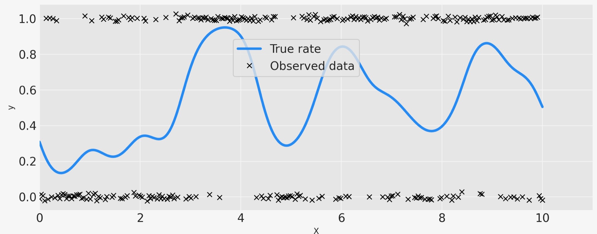
with pm.Model() as model:
    ell = pm.InverseGamma("ell", mu=1.0, sigma=0.5)
    eta = pm.Exponential("eta", lam=1.0)
    cov = eta**2 * pm.gp.cov.ExpQuad(1, ell)

    gp = pm.gp.Latent(cov_func=cov)
    f = gp.prior("f", X=x[:, None])

    # logit link and Bernoulli likelihood
    p = pm.Deterministic("p", pm.math.invlogit(f))
    y_ = pm.Bernoulli("y", p=p, observed=y)

    idata = pm.sample(1000, chains=2, cores=1)
# check Rhat, values above 1 may indicate convergence issues
n_nonconverged = int(np.sum(az.rhat(idata)[["eta", "ell", "f_rotated_"]].to_array() > 1.03).values)
if n_nonconverged == 0:
    print("No Rhat values above 1.03, \N{check mark}")
else:
    print(f"The MCMC chains for {n_nonconverged} RVs appear not to have converged.")
No Rhat values above 1.03, ✓
ax = az.plot_pair(
    idata,
    var_names=["eta", "ell"],
    kind=["kde", "scatter"],
    scatter_kwargs={"color": "darkslategray", "alpha": 0.4},
    gridsize=25,
    divergences=True,
)

ax.axvline(x=eta_true, color="dodgerblue")
ax.axhline(y=ell_true, color="dodgerblue");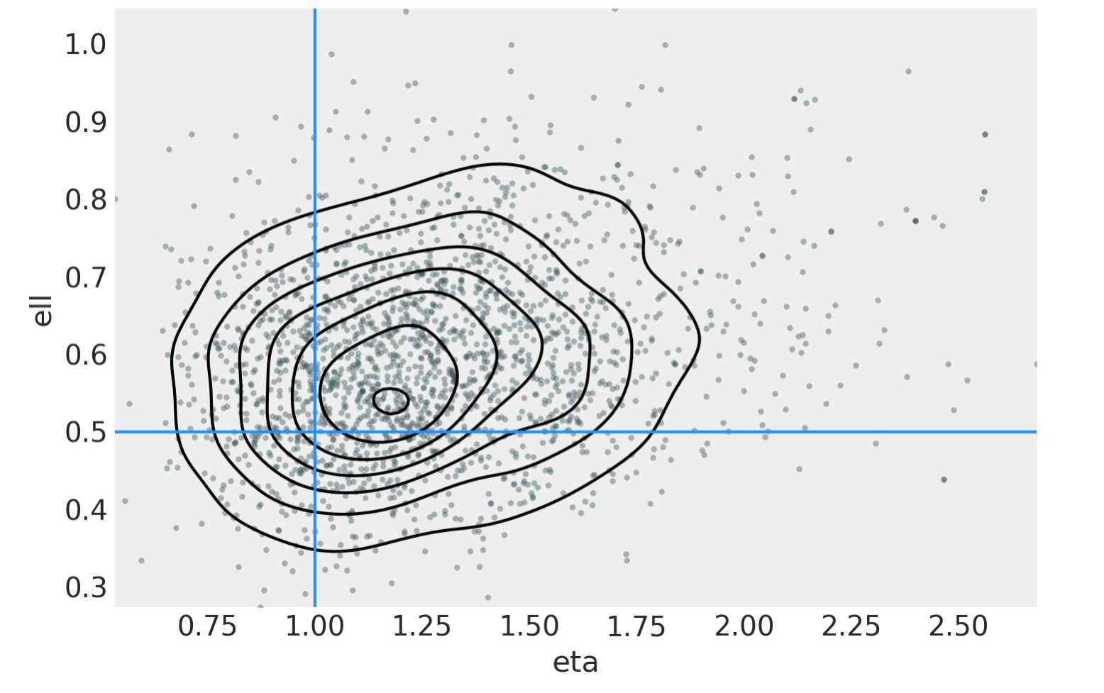
n_pred = 200
X_new = np.linspace(0, 12, n_pred)[:, None]

with model:
    f_pred = gp.conditional("f_pred", X_new, jitter=1e-4)
    p_pred = pm.Deterministic("p_pred", pm.math.invlogit(f_pred))

with model:
    ppc = pm.sample_posterior_predictive(idata.posterior, var_names=["f_pred", "p_pred"])
    idata.extend(ppc)
# plot the results
fig = plt.figure(figsize=(10, 4))
ax = fig.gca()

# plot the samples from the gp posterior with samples and shading
p_pred = az.extract(idata.posterior_predictive, var_names="p_pred").transpose("sample", ...)
plot_gp_dist(ax, p_pred, X_new)

# plot the data (with some jitter) and the true latent function
plt.plot(x, pm.math.invlogit(f_true).eval(), "dodgerblue", lw=3, label="True f")
plt.plot(
    x,
    y + np.random.randn(y.shape[0]) * 0.01,
    "kx",
    ms=6,
    alpha=0.5,
    label="Observed data",
)

# axis labels and title
plt.xlabel("X")
plt.ylabel("True f(x)")
plt.xlim([0, 12])
plt.title("Posterior distribution over $f(x)$ at the observed values")
plt.legend(loc=(0.32, 0.65), frameon=True);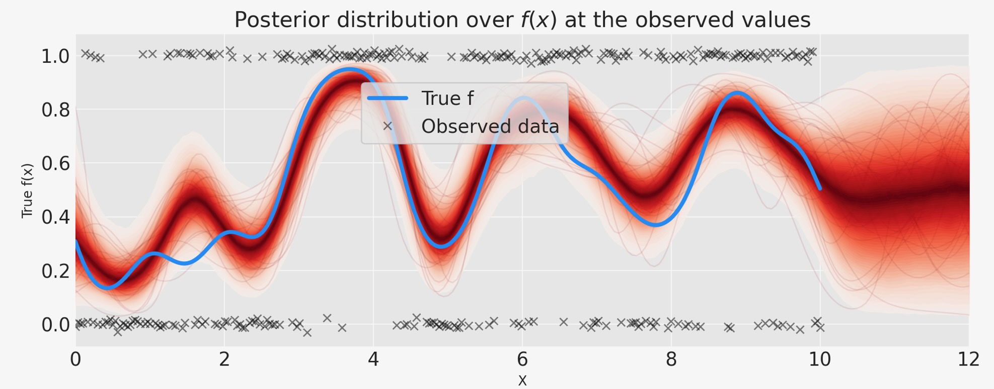
製作者
著者:Bill Engels 2017年
更新:Colin Caroll 2019年
更新:Bill Engels 2022年 9月 PyMC v4
に事前分布を置くことができます。 "潜在”と呼ばれます、なぜなら、GPはそ)