多変量ガウシアン・ランダム・ウォーク

import arviz as az
import matplotlib.pyplot as plt
import numpy as np
import pymc as pm
import pytensor

from scipy.linalg import cholesky

%matplotlib inline

RANDOM_SEED = 8927
rng = np.random.default_rng(RANDOM_SEED)
az.style.use("arviz-darkgrid")

　このノートブックは、多変量ガウシアン・ランダム・ウォーク(GRWs)を使った相関時系列適合の方法を示します。特に、私たちは、GRWsに依存したモデルに対して時系列データのベイジアン回帰を実行します。

　私たちは、３次元時系列としてデータを生成します。

• i -> α_i そして　i -> β_i , i ⊆ {0, 1, 2, 3, 4 }, は、二つの相関行列Σ_α Σ_β のための　二つの３次元ガウシアンランダムウォークです。
• 私たちは、インデックス$ を定義します。

　i[t] = j for t= 60j , 60j+1,...,60j + 59, and j=0,1,2,3,4,$

• *　は私たちが3 x 300 行列のjー番目のカラムとj-番目のベクターj =0,1,2,...299 のエントリーを乗算することを意味します。
• ε_tは iid 正規エントリーN(0,σ² ) の 3x 300行列

　系列yは、ステップ0,60,120,180,240の５度、GRW αのために変化します。その間、yは、GRW βのインクリメントのために　ステップ1,60,120,180,240 で変化します。そして各ステップのβの重みは　t／300です。直感的に、ノイズのあるシステム、それは300ステップの終端を５回経過し時に衝撃を受けます。しかし、βの衝撃の大きさは、段階的に各ステップで大きくなります。

データ生成

データを生成して図示しましょう。

D = 3  # Dimension of random walks
N = 300  # Number of steps
sections = 5  # Number of sections
period = N / sections  # Number steps in each section

Sigma_alpha = rng.standard_normal((D, D))
Sigma_alpha = Sigma_alpha.T.dot(Sigma_alpha)  # Construct covariance matrix for alpha
L_alpha = cholesky(Sigma_alpha, lower=True)  # Obtain its Cholesky decomposition

Sigma_beta = rng.standard_normal((D, D))
Sigma_beta = Sigma_beta.T.dot(Sigma_beta)  # Construct covariance matrix for beta
L_beta = cholesky(Sigma_beta, lower=True)  # Obtain its Cholesky decomposition

# Gaussian random walks:
alpha = np.cumsum(L_alpha.dot(rng.standard_normal((D, sections))), axis=1).T
beta = np.cumsum(L_beta.dot(rng.standard_normal((D, sections))), axis=1).T
t = np.arange(N)[:, None] / N
alpha = np.repeat(alpha, period, axis=0)
beta = np.repeat(beta, period, axis=0)
# Correlated series
sigma = 0.1
y = alpha + beta * t + sigma * rng.standard_normal((N, 1))

# Plot the correlated series
plt.figure(figsize=(12, 5))
plt.plot(t, y, ".", markersize=2, label=("y_0 data", "y_1 data", "y_2 data"))
plt.title("Three Correlated Series")
plt.xlabel("Time")
plt.legend()
plt.show();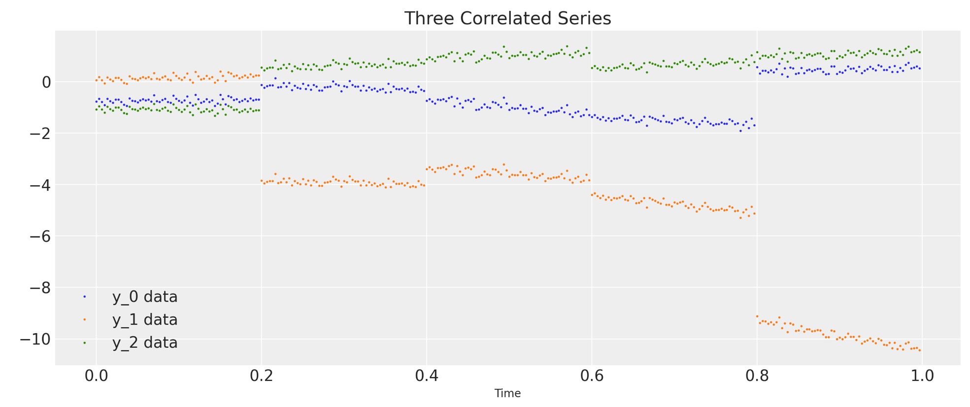

モデル

　最初に私たちは、サンプリングの前に私たちのデータと時間パラメータを、再スケール化するためにスケーリングクラスを紹介します。その後、スケールされていないデータにマッチするために予測を再スケールします。

class Scaler:
    def __init__(self):
        mean_ = None
        std_ = None

    def transform(self, x):
        return (x - self.mean_) / self.std_

    def fit_transform(self, x):
        self.mean_ = x.mean(axis=0)
        self.std_ = x.std(axis=0)
        return self.transform(x)

    def inverse_transform(self, x):
        return x * self.std_ + self.mean_

　私たちは、ここでGRWs のαとβ、標準偏差σ、コレスキー行列のハイパーパラメータの 事前分布を果たす回帰モデルを構築します。私たちは、コレスキー行列のためにLKJ事前分布[Lewandowski et al., 2009 参考文献]を使います。(以下のコレスキー共分散の記事を参照してください。）

def inference(t, y, sections, n_samples=100):
    N, D = y.shape

    # Standardize y and t
    y_scaler = Scaler()
    t_scaler = Scaler()
    y = y_scaler.fit_transform(y)
    t = t_scaler.fit_transform(t)
    # Create a section index
    t_section = np.repeat(np.arange(sections), N / sections)

    # Create PyTensor equivalent
    t_t = pytensor.shared(np.repeat(t, D, axis=1))
    y_t = pytensor.shared(y)
    t_section_t = pytensor.shared(t_section)

    coords = {"y_": ["y_0", "y_1", "y_2"], "steps": np.arange(N)}
    with pm.Model(coords=coords) as model:
        # Hyperpriors on Cholesky matrices
        chol_alpha, *_ = pm.LKJCholeskyCov(
            "chol_cov_alpha", n=D, eta=2, sd_dist=pm.HalfCauchy.dist(2.5), compute_corr=True
        )
        chol_beta, *_ = pm.LKJCholeskyCov(
            "chol_cov_beta", n=D, eta=2, sd_dist=pm.HalfCauchy.dist(2.5), compute_corr=True
        )

        # Priors on Gaussian random walks
        alpha = pm.MvGaussianRandomWalk(
            "alpha", mu=np.zeros(D), chol=chol_alpha, shape=(sections, D)
        )
        beta = pm.MvGaussianRandomWalk("beta", mu=np.zeros(D), chol=chol_beta, shape=(sections, D))

        # Deterministic construction of the correlated random walk
        alpha_r = alpha[t_section_t]
        beta_r = beta[t_section_t]
        regression = alpha_r + beta_r * t_t

        # Prior on noise ξ
        sigma = pm.HalfNormal("sigma", 1.0)

        # Likelihood
        likelihood = pm.Normal("y", mu=regression, sigma=sigma, observed=y_t, dims=("steps", "y_"))

        # MCMC sampling
        trace = pm.sample(n_samples, tune=1000, chains=4, target_accept=0.9)

        # Posterior predictive sampling
        pm.sample_posterior_predictive(trace, extend_inferencedata=True)

    return trace, y_scaler, t_scaler, t_section

推定

　私たちは、モデルからサンプルします。そしてトレース、時間と空間のためのスケーリング関数、スケールされた時間にインデックスをリターンします。

trace, y_scaler, t_scaler, t_section = inference(t, y, sections)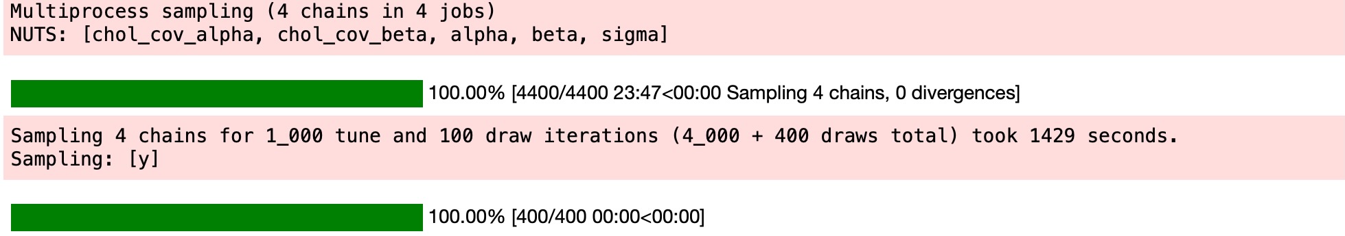

　私たちは、モデルの収束を視覚チェックのためにarviz.plot_energy()を使ってエナジープロットを表示します。その後、arviz.plot_ppc()を使い、私たちは、観測データyに対して、事後予測サンプルの分布を図示します。この図はモデル（yの値は実際に、yのスケールされたバージョンに一致することに注意してください）の正確さの一般的な考えを提供します。

az.plot_energy(trace)
az.plot_ppc(trace);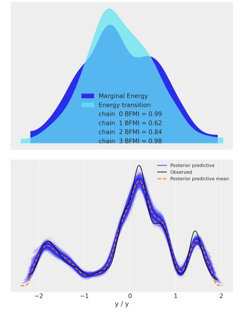

事後分布可視化

　上のグラフはよく見えます。ここで、私たちは予測した３次元系列の平均に対して、観測した３次元系列を図示します。言い換えると、私たちはモデルから予測した回帰線に対してデータを図示します。

# Compute the predicted mean of the multivariate GRWs
alpha_mean = trace.posterior["alpha"].mean(dim=("chain", "draw"))
beta_mean = trace.posterior["beta"].mean(dim=("chain", "draw"))

# Compute the predicted mean of the correlated series
y_pred = y_scaler.inverse_transform(
    alpha_mean[t_section].values + beta_mean[t_section].values * t_scaler.transform(t)
)

# Plot the predicted mean
fig, ax = plt.subplots(1, 1, figsize=(12, 6))
ax.plot(t, y, ".", markersize=2, label=("y_0 data", "y_1 data", "y_2 data"))
plt.gca().set_prop_cycle(None)
ax.plot(t, y_pred, label=("y_0 pred", "y_1 pred", "y_2 pred"))
ax.set_xlabel("Time")
ax.legend()
ax.set_title("Predicted Mean of Three Correlated Series");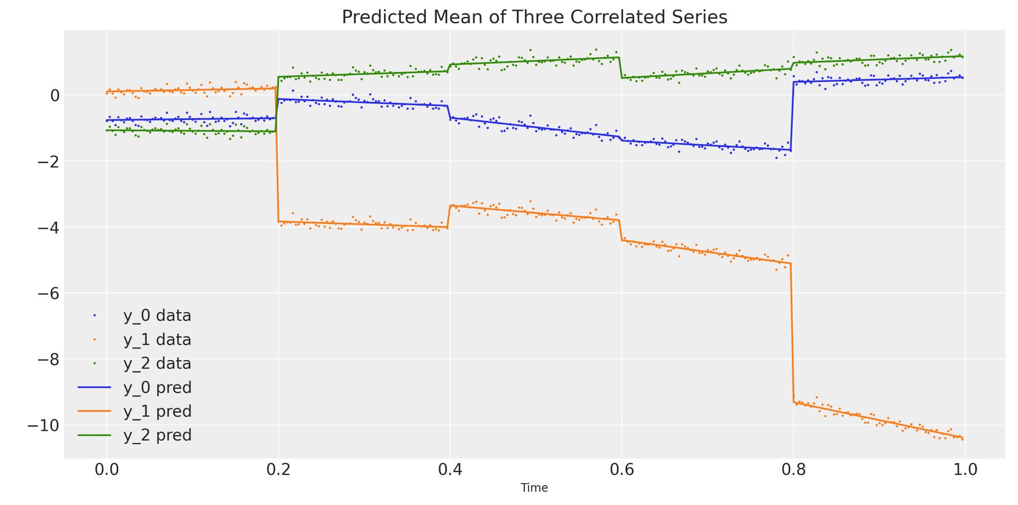

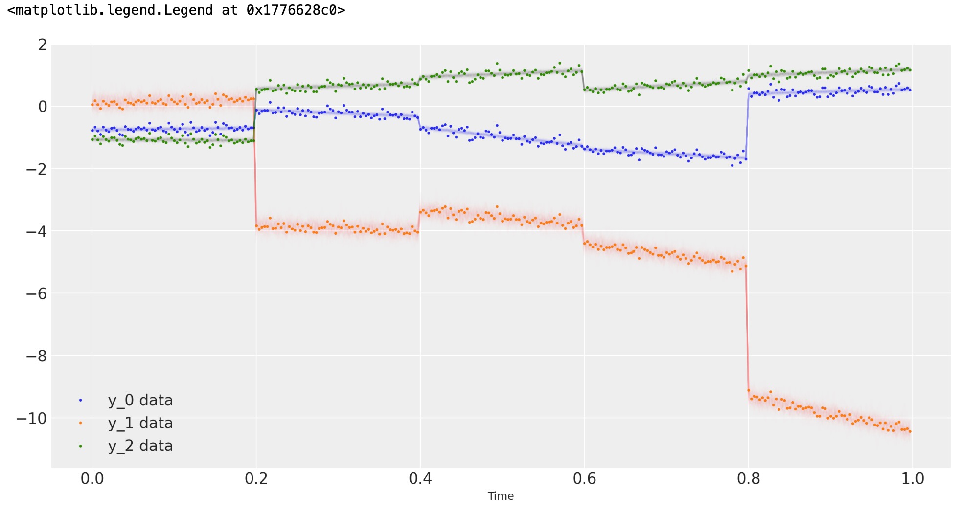
　最後に、私たちは事後予測サンプルに対してデータを図示します。

# Rescale the posterior predictive samples
ppc_y = y_scaler.inverse_transform(trace.posterior_predictive["y"].mean("chain"))

fig, ax = plt.subplots(1, 1, figsize=(12, 6))
# Plot the data
ax.plot(t, y, ".", markersize=3, label=("y_0 data", "y_1 data", "y_2 data"))
# Plot the posterior predictive samples
ax.plot(t, ppc_y.sel(y_="y_0").T, color="C0", alpha=0.003)
ax.plot(t, ppc_y.sel(y_="y_1").T, color="C1", alpha=0.003)
ax.plot(t, ppc_y.sel(y_="y_2").T, color="C2", alpha=0.003)
ax.set_xlabel("Time")
ax.legend()