IrisデータセットのSVM分類の相違の図示

irisデータセットの2D投影図の異なる線形SVM分類を比較します。私たちは、このデータセットの最初の二つの特徴を考慮するだけです。

• 萼片(花の）の長さ
• 萼片の幅

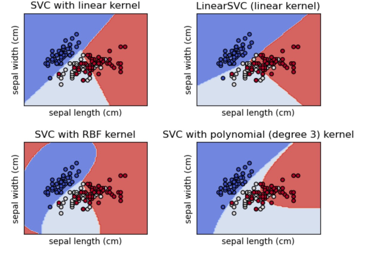
この例は、異なるカーネルによる四つのSVM分類のための決定面を図示する方法を示します。

線形モデルLinearSVC()とSVC(kernel='linear')はわずかに異なる決定境界に分岐します。これは、以下の相違による結果とされます。

• SVCは通常のヒンジ損失を最小化させますが、LinearSVCは、ヒンジ損失の二乗を最小化します。
• SVCは１対１の多重分類縮約しますが、LinearSVMは、1対全て(1対残りとしても知られています)多重分類縮約を使います。

　非線形のカーネルモデル(多項式、またはガウシアンRBF)は、もっと柔軟な、カーネルの種類とそのパラメータに依存したシェイプの非線形決定境界を持ちますが、両方の線形モデルは、線形の決定境界を持ちます。

import matplotlib.pyplot as plt

from sklearn import datasets, svm
from sklearn.inspection import DecisionBoundaryDisplay

# import some data to play with
iris = datasets.load_iris()
# Take the first two features. We could avoid this by using a two-dim dataset
X = iris.data[:, :2]
y = iris.target

# we create an instance of SVM and fit out data. We do not scale our
# data since we want to plot the support vectors
C = 1.0  # SVM regularization parameter
models = (
    svm.SVC(kernel="linear", C=C),
    svm.LinearSVC(C=C, max_iter=10000, dual=True),
    svm.SVC(kernel="rbf", gamma=0.7, C=C),
    svm.SVC(kernel="poly", degree=3, gamma="auto", C=C),
)
models = (clf.fit(X, y) for clf in models)

# title for the plots
titles = (
    "SVC with linear kernel",
    "LinearSVC (linear kernel)",
    "SVC with RBF kernel",
    "SVC with polynomial (degree 3) kernel",
)

# Set-up 2x2 grid for plotting.
fig, sub = plt.subplots(2, 2)
plt.subplots_adjust(wspace=0.4, hspace=0.4)

X0, X1 = X[:, 0], X[:, 1]

for clf, title, ax in zip(models, titles, sub.flatten()):
    disp = DecisionBoundaryDisplay.from_estimator(
        clf,
        X,
        response_method="predict",
        cmap=plt.cm.coolwarm,
        alpha=0.8,
        ax=ax,
        xlabel=iris.feature_names[0],
        ylabel=iris.feature_names[1],
    )
    ax.scatter(X0, X1, c=y, cmap=plt.cm.coolwarm, s=20, edgecolors="k")
    ax.set_xticks(())
    ax.set_yticks(())
    ax.set_title(title)

plt.show()