外れ値検知のためのアノマリー検知アルゴリズムの比較

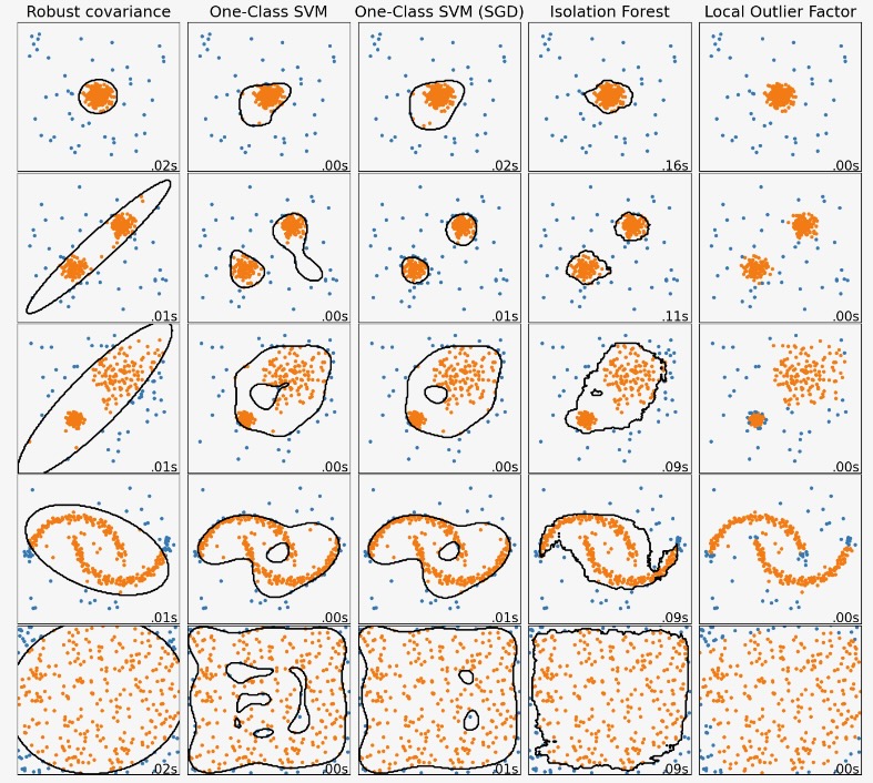
　この例は、２Dデータセットの異なるアノマリー検知アルゴリズムの性質を示します。データセットは多様な様式のデータを処理するためのアルゴリズムの能力を説明するために二つか三つのモード（高密度の領域）を含みます。

　各データセットは、サンプルの１５％がランダムな一様ノイズとして生成されます。この目的は、OneClassSVMのnuパラメータで与えられる値と他の外れ値検知アルゴリズムの（不純物が含まれる）汚染されたパラメータの値です。外れ値検知で使われる時に、新しいデータに適用される予測法を持たない局所外れ因子(LOF)をのぞいて、外れ値と内部の境界の決定は、黒で表記されます。

　OneClassSVMは、外れ値に敏感であると知られています。そしてこのように外れ値検知に対しては、あまりうまく実行しません。この推定はトレーニングセットが外れ値で汚染されていない時に、目新しさ検知のもっともよい方法になります。いわば、高次の外れ値検知や、または内部データ分布のいくつかの仮定がない時は、非常に難問になります。そして、OneClassSVMは、ハイパーパラメータの値に依存したこれらの状況では、役立つ結果を与えるかもしれません。

　sklearn.linear_model.SGDOneClassSVMは、確率的勾配下降に基づくOneClass SVMの実装です。カーネル近似を組み合わせてこの推定は、カーネル化　sklearn.svm.OneClassSVMのソリューションを近似することに使うことができます。私たちは、区別できませんが、sklearn.linear_model.SGDOneClassSVMとsklearn.svm.OneClassSVMの一つの決定境界はとても似ています。sklearn.leinear_model.SDGONeClassSVMを使う主要な利点は、サンプル数に応じて線形にスケールすることです。

　sklearn.covariate.EllipticEnvelopeは、データがガウシアンで、楕円を学習することを仮定します。データが一様でないときは、このように品質を下げます。しかし、この推定は外れ値に堅牢であることを注意してください。

　IsolationForestとLocalOutlierFactorは、多様な様式のデータセットに妥当に良く実行しているようです。LocalOutlierFactorの他の推定を超える利点は、二つのモードが異なる密度を持っている三つ目のデータセットで示されます。この利点は、一つのサンプルの異常なスコアを、その近傍のスコアと比較するだけであることを意味するLOFの局所的な様相で説明されます。

　最後に、最後のデータセットでは、それらがハイパーキューブ内に一様に分布しているので、一つのサンプルが、他のサンプルより異常であると判断するのが困難です。少し過度に適合するOneClassSVM以外、全ての推定はこの状況のために、解決法が低下することを表しています。そのようなケースでは、良い推定は全てのサンプルに同様のスコアを割り当てるので、サンプルの異常さのスコアをもっと密接に見ることが賢明になります。

　これらの例は、アルゴリズムについて何らかの直感を与えますが、この直感はとても高い次元のデータには適用しないかもしれません。

　最後に、モデルのパラメータは、ここでは手動で設定しており、しかしそれは演習なので、それらは調整する必要があることに気をつけてください。ラベルデータの欠如は、問題が完全に教師なし（unsupervised）なので、モデルの選択は難題になります。

# Author: Alexandre Gramfort <alexandre.gramfort@inria.fr>
#         Albert Thomas <albert.thomas@telecom-paristech.fr>
# License: BSD 3 clause

import time

import numpy as np
import matplotlib
import matplotlib.pyplot as plt

from sklearn import svm
from sklearn.datasets import make_moons, make_blobs
from sklearn.covariance import EllipticEnvelope
from sklearn.ensemble import IsolationForest
from sklearn.neighbors import LocalOutlierFactor
from sklearn.linear_model import SGDOneClassSVM
from sklearn.kernel_approximation import Nystroem
from sklearn.pipeline import make_pipeline

matplotlib.rcParams["contour.negative_linestyle"] = "solid"

# Example settings
n_samples = 300
outliers_fraction = 0.15
n_outliers = int(outliers_fraction * n_samples)
n_inliers = n_samples - n_outliers

# define outlier/anomaly detection methods to be compared.
# the SGDOneClassSVM must be used in a pipeline with a kernel approximation
# to give similar results to the OneClassSVM
anomaly_algorithms = [
    (
        "Robust covariance",
        EllipticEnvelope(contamination=outliers_fraction, random_state=42),
    ),
    ("One-Class SVM", svm.OneClassSVM(nu=outliers_fraction, kernel="rbf", gamma=0.1)),
    (
        "One-Class SVM (SGD)",
        make_pipeline(
            Nystroem(gamma=0.1, random_state=42, n_components=150),
            SGDOneClassSVM(
                nu=outliers_fraction,
                shuffle=True,
                fit_intercept=True,
                random_state=42,
                tol=1e-6,
            ),
        ),
    ),
    (
        "Isolation Forest",
        IsolationForest(contamination=outliers_fraction, random_state=42),
    ),
    (
        "Local Outlier Factor",
        LocalOutlierFactor(n_neighbors=35, contamination=outliers_fraction),
    ),
]

# Define datasets
blobs_params = dict(random_state=0, n_samples=n_inliers, n_features=2)
datasets = [
    make_blobs(centers=[[0, 0], [0, 0]], cluster_std=0.5, **blobs_params)[0],
    make_blobs(centers=[[2, 2], [-2, -2]], cluster_std=[0.5, 0.5], **blobs_params)[0],
    make_blobs(centers=[[2, 2], [-2, -2]], cluster_std=[1.5, 0.3], **blobs_params)[0],
    4.0
    * (
        make_moons(n_samples=n_samples, noise=0.05, random_state=0)[0]
        - np.array([0.5, 0.25])
    ),
    14.0 * (np.random.RandomState(42).rand(n_samples, 2) - 0.5),
]

# Compare given classifiers under given settings
xx, yy = np.meshgrid(np.linspace(-7, 7, 150), np.linspace(-7, 7, 150))

plt.figure(figsize=(len(anomaly_algorithms) * 2 + 4, 12.5))
plt.subplots_adjust(
    left=0.02, right=0.98, bottom=0.001, top=0.96, wspace=0.05, hspace=0.01
)

plot_num = 1
rng = np.random.RandomState(42)

for i_dataset, X in enumerate(datasets):
    # Add outliers
    X = np.concatenate([X, rng.uniform(low=-6, high=6, size=(n_outliers, 2))], axis=0)

    for name, algorithm in anomaly_algorithms:
        t0 = time.time()
        algorithm.fit(X)
        t1 = time.time()
        plt.subplot(len(datasets), len(anomaly_algorithms), plot_num)
        if i_dataset == 0:
            plt.title(name, size=18)

        # fit the data and tag outliers
        if name == "Local Outlier Factor":
            y_pred = algorithm.fit_predict(X)
        else:
            y_pred = algorithm.fit(X).predict(X)

        # plot the levels lines and the points
        if name != "Local Outlier Factor":  # LOF does not implement predict
            Z = algorithm.predict(np.c_[xx.ravel(), yy.ravel()])
            Z = Z.reshape(xx.shape)
            plt.contour(xx, yy, Z, levels=[0], linewidths=2, colors="black")

        colors = np.array(["#377eb8", "#ff7f00"])
        plt.scatter(X[:, 0], X[:, 1], s=10, color=colors[(y_pred + 1) // 2])

        plt.xlim(-7, 7)
        plt.ylim(-7, 7)
        plt.xticks(())
        plt.yticks(())
        plt.text(
            0.99,
            0.01,
            ("%.2fs" % (t1 - t0)).lstrip("0"),
            transform=plt.gca().transAxes,
            size=15,
            horizontalalignment="right",
        )
        plot_num += 1

plt.show()