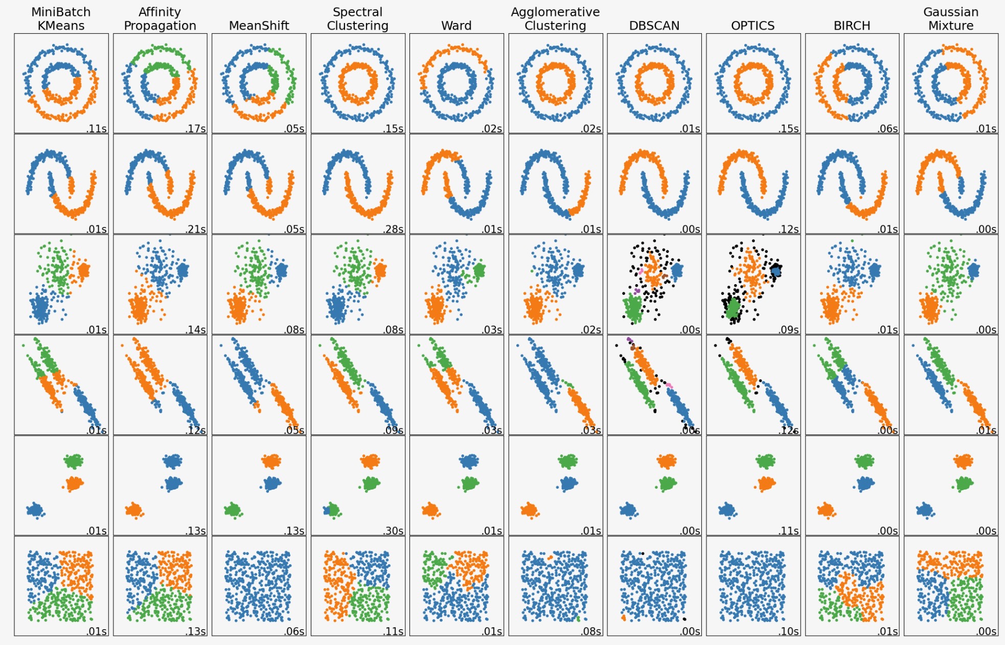
この例は、”興味深い”が2Dのデータセット上で異なるクラスタリングアルゴリズムの性質を示します。最後のデータセットの例外で、これらのデータセットアルゴリズムペアの各パラメータは、良いクラスタリング結果を生み出すために調整されます。いくつかのアルゴリズムは、他のものよりパラメータの値にもっと敏感です。
最後のデータセットは、クラスタリングの"null"状況の例です。そのデータは均一で、良いクラスタリングはありません。この例のために、nullデータセットは、上の例の列のデータセットとして、同じパラメータを使います。それは、データ構造とパラメータ値のミスマッチを表しています。
import time
import warnings

import numpy as np
import matplotlib.pyplot as plt

from sklearn import cluster, datasets, mixture
from sklearn.neighbors import kneighbors_graph
from sklearn.preprocessing import StandardScaler
from itertools import cycle, islice

np.random.seed(0)

# ============
# Generate datasets. We choose the size big enough to see the scalability
# of the algorithms, but not too big to avoid too long running times
# ============
n_samples = 500
noisy_circles = datasets.make_circles(n_samples=n_samples, factor=0.5, noise=0.05)
noisy_moons = datasets.make_moons(n_samples=n_samples, noise=0.05)
blobs = datasets.make_blobs(n_samples=n_samples, random_state=8)
no_structure = np.random.rand(n_samples, 2), None

# Anisotropicly distributed data
random_state = 170
X, y = datasets.make_blobs(n_samples=n_samples, random_state=random_state)
transformation = [[0.6, -0.6], [-0.4, 0.8]]
X_aniso = np.dot(X, transformation)
aniso = (X_aniso, y)

# blobs with varied variances
varied = datasets.make_blobs(
    n_samples=n_samples, cluster_std=[1.0, 2.5, 0.5], random_state=random_state
)

# ============
# Set up cluster parameters
# ============
plt.figure(figsize=(9 * 2 + 3, 13))
plt.subplots_adjust(
    left=0.02, right=0.98, bottom=0.001, top=0.95, wspace=0.05, hspace=0.01
)

plot_num = 1

default_base = {
    "quantile": 0.3,
    "eps": 0.3,
    "damping": 0.9,
    "preference": -200,
    "n_neighbors": 3,
    "n_clusters": 3,
    "min_samples": 7,
    "xi": 0.05,
    "min_cluster_size": 0.1,
}

datasets = [
    (
        noisy_circles,
        {
            "damping": 0.77,
            "preference": -240,
            "quantile": 0.2,
            "n_clusters": 2,
            "min_samples": 7,
            "xi": 0.08,
        },
    ),
    (
        noisy_moons,
        {
            "damping": 0.75,
            "preference": -220,
            "n_clusters": 2,
            "min_samples": 7,
            "xi": 0.1,
        },
    ),
    (
        varied,
        {
            "eps": 0.18,
            "n_neighbors": 2,
            "min_samples": 7,
            "xi": 0.01,
            "min_cluster_size": 0.2,
        },
    ),
    (
        aniso,
        {
            "eps": 0.15,
            "n_neighbors": 2,
            "min_samples": 7,
            "xi": 0.1,
            "min_cluster_size": 0.2,
        },
    ),
    (blobs, {"min_samples": 7, "xi": 0.1, "min_cluster_size": 0.2}),
    (no_structure, {}),
]

for i_dataset, (dataset, algo_params) in enumerate(datasets):
    # update parameters with dataset-specific values
    params = default_base.copy()
    params.update(algo_params)

    X, y = dataset

    # normalize dataset for easier parameter selection
    X = StandardScaler().fit_transform(X)

    # estimate bandwidth for mean shift
    bandwidth = cluster.estimate_bandwidth(X, quantile=params["quantile"])

    # connectivity matrix for structured Ward
    connectivity = kneighbors_graph(
        X, n_neighbors=params["n_neighbors"], include_self=False
    )
    # make connectivity symmetric
    connectivity = 0.5 * (connectivity + connectivity.T)

    # ============
    # Create cluster objects
    # ============
    ms = cluster.MeanShift(bandwidth=bandwidth, bin_seeding=True)
    two_means = cluster.MiniBatchKMeans(n_clusters=params["n_clusters"], n_init="auto")
    ward = cluster.AgglomerativeClustering(
        n_clusters=params["n_clusters"], linkage="ward", connectivity=connectivity
    )
    spectral = cluster.SpectralClustering(
        n_clusters=params["n_clusters"],
        eigen_solver="arpack",
        affinity="nearest_neighbors",
    )
    dbscan = cluster.DBSCAN(eps=params["eps"])
    optics = cluster.OPTICS(
        min_samples=params["min_samples"],
        xi=params["xi"],
        min_cluster_size=params["min_cluster_size"],
    )
    affinity_propagation = cluster.AffinityPropagation(
        damping=params["damping"], preference=params["preference"], random_state=0
    )
    average_linkage = cluster.AgglomerativeClustering(
        linkage="average",
        metric="cityblock",
        n_clusters=params["n_clusters"],
        connectivity=connectivity,
    )
    birch = cluster.Birch(n_clusters=params["n_clusters"])
    gmm = mixture.GaussianMixture(
        n_components=params["n_clusters"], covariance_type="full"
    )

    clustering_algorithms = (
        ("MiniBatch\nKMeans", two_means),
        ("Affinity\nPropagation", affinity_propagation),
        ("MeanShift", ms),
        ("Spectral\nClustering", spectral),
        ("Ward", ward),
        ("Agglomerative\nClustering", average_linkage),
        ("DBSCAN", dbscan),
        ("OPTICS", optics),
        ("BIRCH", birch),
        ("Gaussian\nMixture", gmm),
    )

    for name, algorithm in clustering_algorithms:
        t0 = time.time()

        # catch warnings related to kneighbors_graph
        with warnings.catch_warnings():
            warnings.filterwarnings(
                "ignore",
                message="the number of connected components of the "
                + "connectivity matrix is [0-9]{1,2}"
                + " > 1. Completing it to avoid stopping the tree early.",
                category=UserWarning,
            )
            warnings.filterwarnings(
                "ignore",
                message="Graph is not fully connected, spectral embedding"
                + " may not work as expected.",
                category=UserWarning,
            )
            algorithm.fit(X)

        t1 = time.time()
        if hasattr(algorithm, "labels_"):
            y_pred = algorithm.labels_.astype(int)
        else:
            y_pred = algorithm.predict(X)

        plt.subplot(len(datasets), len(clustering_algorithms), plot_num)
        if i_dataset == 0:
            plt.title(name, size=18)

        colors = np.array(
            list(
                islice(
                    cycle(
                        [
                            "#377eb8",
                            "#ff7f00",
                            "#4daf4a",
                            "#f781bf",
                            "#a65628",
                            "#984ea3",
                            "#999999",
                            "#e41a1c",
                            "#dede00",
                        ]
                    ),
                    int(max(y_pred) + 1),
                )
            )
        )
        # add black color for outliers (if any)
        colors = np.append(colors, ["#000000"])
        plt.scatter(X[:, 0], X[:, 1], s=10, color=colors[y_pred])

        plt.xlim(-2.5, 2.5)
        plt.ylim(-2.5, 2.5)
        plt.xticks(())
        plt.yticks(())
        plt.text(
            0.99,
            0.01,
            ("%.2fs" % (t1 - t0)).lstrip("0"),
            transform=plt.gca().transAxes,
            size=15,
            horizontalalignment="right",
        )
        plot_num += 1

plt.show()