DBSCAN(Density-Based Spatial Clustering Applications with Noise)は、高い密度の領域内でのコアのサンプルを見つけます。そしてそれらからクラスターに拡張します。このアルゴリズムは、同様の密度のクラスターを含んでいるデータに適しています。
2Dデータセットでの異なるクラスタリングアルゴリズムのデモ "toyデータセットでの異なるクラスタリングアルゴリズムの比較(ハイパーリンク)" の例を参照してください。
データ生成
私たちは、三つの合成クラスターを作るためにmake_blobsを使います。
from sklearn.datasets import make_blobs
from sklearn.preprocessing import StandardScaler

centers = [[1, 1], [-1, -1], [1, -1]]
X, labels_true = make_blobs(
    n_samples=750, centers=centers, cluster_std=0.4, random_state=0
)

X = StandardScaler().fit_transform(X)
私たちは、結果のデータを可視化できます。
import matplotlib.pyplot as plt

plt.scatter(X[:, 0], X[:, 1])
plt.show()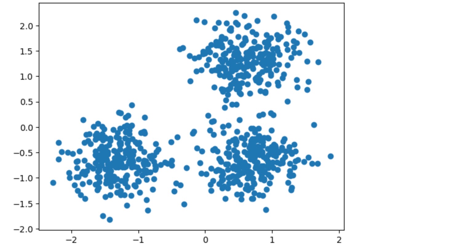
DBSCANの計算
labels_属性を使って、DBSCANによって割り当てられたラベルにアクセスできます。ノイズのあるサンプルはラベルmath:-1で与えられます。
import numpy as np
from sklearn.cluster import DBSCAN
from sklearn import metrics

db = DBSCAN(eps=0.3, min_samples=10).fit(X)
labels = db.labels_

# Number of clusters in labels, ignoring noise if present.
n_clusters_ = len(set(labels)) - (1 if -1 in labels else 0)
n_noise_ = list(labels).count(-1)

print("Estimated number of clusters: %d" % n_clusters_)
print("Estimated number of noise points: %d" % n_noise_)
Estimated number of clusters: 3
Estimated number of noise points: 18クラスタリングアルゴリズムは基本的に教師なし学習法です。しかし、make_blobsは合成クラスタへの真のラベルへのアクセスを与えるので、クラスターの結果の品質の量を測るために、この"教師付き"の敷地の真の情報の影響度の評価に使うことができます。そのような計測の例は、同質性、完全性、V-尺度、Rand-インデックス、適合Rand-インデックス、適合相互情報(AMI)があります。
もし、敷地の真のラベルがわからないならば、評価はモデルの結果それ自身を使ってだけ実行できます。このケースでは、Silhouette係数が役立ちます。
もっと詳しい情報は、"クラスタリングパフォーマンスの評価での機会の適合(ハイパーリンク)"例、または、"クラスタリングパフォーマンス評価(ハイパーリンク)"モジュールを参照してください。
print(f"Homogeneity: {metrics.homogeneity_score(labels_true, labels):.3f}")
print(f"Completeness: {metrics.completeness_score(labels_true, labels):.3f}")
print(f"V-measure: {metrics.v_measure_score(labels_true, labels):.3f}")
print(f"Adjusted Rand Index: {metrics.adjusted_rand_score(labels_true, labels):.3f}")
print(
    "Adjusted Mutual Information:"
    f" {metrics.adjusted_mutual_info_score(labels_true, labels):.3f}"
)
print(f"Silhouette Coefficient: {metrics.silhouette_score(X, labels):.3f}")
Homogeneity: 0.953
Completeness: 0.883
V-measure: 0.917
Adjusted Rand Index: 0.952
Adjusted Mutual Information: 0.916
Silhouette Coefficient: 0.626結果の図示
コアサンプル(大きなドット)とコアでないサンプル(小さなドット)は割り当てられたクラスターに応じた色で符号化されています。ノイズとしてタグ付けられたサンプルは黒で表記されます。
unique_labels = set(labels)
core_samples_mask = np.zeros_like(labels, dtype=bool)
core_samples_mask[db.core_sample_indices_] = True

colors = [plt.cm.Spectral(each) for each in np.linspace(0, 1, len(unique_labels))]
for k, col in zip(unique_labels, colors):
    if k == -1:
        # Black used for noise.
        col = [0, 0, 0, 1]

    class_member_mask = labels == k

    xy = X[class_member_mask & core_samples_mask]
    plt.plot(
        xy[:, 0],
        xy[:, 1],
        "o",
        markerfacecolor=tuple(col),
        markeredgecolor="k",
        markersize=14,
    )

    xy = X[class_member_mask & ~core_samples_mask]
    plt.plot(
        xy[:, 0],
        xy[:, 1],
        "o",
        markerfacecolor=tuple(col),
        markeredgecolor="k",
        markersize=6,
    )

plt.title(f"Estimated number of clusters: {n_clusters_}")
plt.show()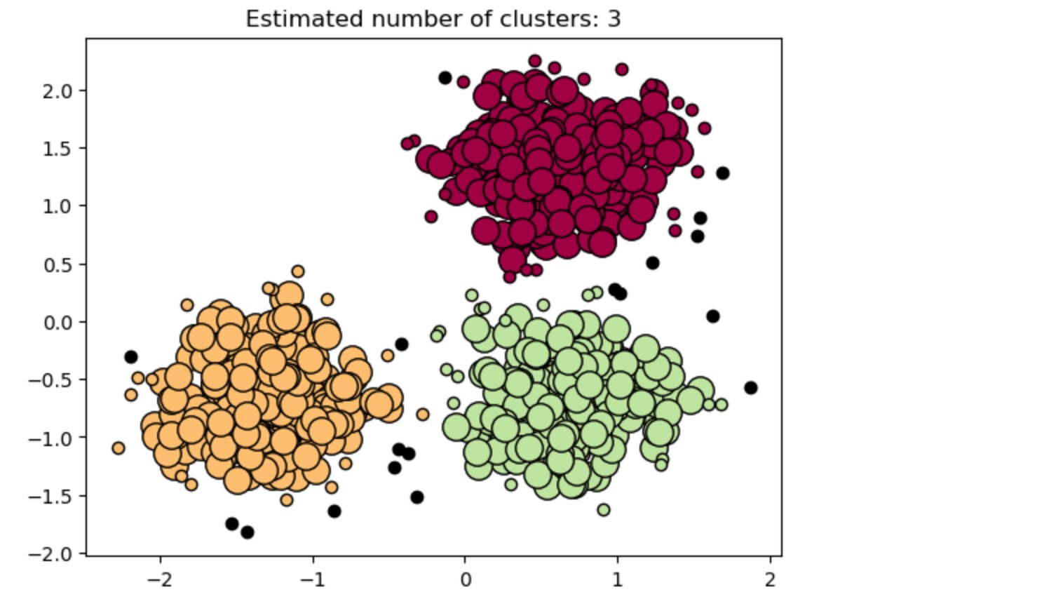
は、高い密度の領域内でのコアのサンプルを見つけます。そしてそれらからク )