ロバスト共分散推定とマハラノビス距離の関連性

　この例はガウス分布データのマハラノビス距離での共分散の推定を示します。

　ガウス分布データでは、分布のモードへの観測値x_i の距離はマハラノビス距離を使って計算できます。

　ここで、μとΣは、ガウス分布下での位置と共分散です。

　実際は、μとΣは任意の推定で取り替えられます。標準共分散最大尤度推定(MLE)は、データセットの外れ値の存在に対して非常に敏感です。それゆえ、下側のマハラノビス距離もまた同様です。推定がデータセットのエラーの観測に抵抗があること、計算したマハラノビス距離が観測の真の観測を正確に反映していることを保証するために、ロバスト共分散推定を使う方が良いでしょう。

　最小の共分散決定因子推定(MCD)は、堅牢、共分散の高ブレークダウンポイント(すなわち、高く(不純物で)汚染されたデータセット、外れ値が　(n _samples - n _features)/2 まで 、共分散行列を推定することができます)推定です。MCDの背後にある考えは、(n _samples - n _features + 1 ) / 2 の観測値を見つけることです。その観測値の実証的な共分散は、位置と共分散の標準の推定を計算して観測値の純粋なサブセットを分離している、少数の決定因子を持ちます。MCDは　P.J.Rousseuw [注1] によって紹介されました。

　この例はどのようにマハラノビス距離が、外れデータによって影響されるかを説明しています。汚染された分布から出力される観測値は、マハラノビス距離を元にした標準共分散MLEを使った時のガウス分布である現実の観測値から区別できるものではありません。MCDを元にしたマハラノビス距離を使うことで、二つの量を区別できます。関連のアプリケーションは、外れ値検知、観測順位、クラスタリングを含みます。

データの生成

　最初に、１２５のサンプルと二つの特徴のデータセットを生成します。両方の特徴は、平均が０のガウス分布で、特徴１は標準偏差が２に等しく、特徴２は標準偏差が１になります。次に、２５サンプルがガウス外れ値サンプルに取り替えられます。そのサンプルは、特徴１が標準偏差１で特徴２が標準偏差７に等しいものです。

import numpy as np

# for consistent results
np.random.seed(7)

n_samples = 125
n_outliers = 25
n_features = 2

# generate Gaussian data of shape (125, 2)
gen_cov = np.eye(n_features)
gen_cov[0, 0] = 2.0
X = np.dot(np.random.randn(n_samples, n_features), gen_cov)
# add some outliers
outliers_cov = np.eye(n_features)
outliers_cov[np.arange(1, n_features), np.arange(1, n_features)] = 7.0
X[-n_outliers:] = np.dot(np.random.randn(n_outliers, n_features), outliers_cov)

結果の比較

　下に、MCDとMLEを元にした共分散推定を私たちのデータに適合させ、推定した共分散行列を出力しています。推定した特徴２の分散は、MLEを元にした推定が、MCDロバスト推定(1.2)よりもずっと高いことに注意してください。これは、MCDを元にしたロバスト推定が、もっとずっと外れ値サンプルに耐性があることを示しています。そのサンプルは特徴２でもっと大きい分散を持つよう設計されています。

import matplotlib.pyplot as plt
from sklearn.covariance import EmpiricalCovariance, MinCovDet

# fit a MCD robust estimator to data
robust_cov = MinCovDet().fit(X)
# fit a MLE estimator to data
emp_cov = EmpiricalCovariance().fit(X)
print(
    "Estimated covariance matrix:\nMCD (Robust):\n{}\nMLE:\n{}".format(
        robust_cov.covariance_, emp_cov.covariance_
    )
)

Estimated covariance matrix:
MCD (Robust):
[[ 3.26253567e+00 -3.06695631e-03]
 [-3.06695631e-03  1.22747343e+00]]
MLE:
[[ 3.23773583 -0.24640578]
 [-0.24640578  7.51963999]]

　相違をもっとよく可視化するために、私たちは、両方の方法で計算されたマハラノビス距離の外形を図示します。ロバストMCDに基づくマハラノビス距離は、内側の黒い点によく適合します。それは、MLEに基づく距離は、外れ値の赤い点によってもっと影響を受けることに注意してください。

fig, ax = plt.subplots(figsize=(10, 5))
# Plot data set
inlier_plot = ax.scatter(X[:, 0], X[:, 1], color="black", label="inliers")
outlier_plot = ax.scatter(
    X[:, 0][-n_outliers:], X[:, 1][-n_outliers:], color="red", label="outliers"
)
ax.set_xlim(ax.get_xlim()[0], 10.0)
ax.set_title("Mahalanobis distances of a contaminated data set")

# Create meshgrid of feature 1 and feature 2 values
xx, yy = np.meshgrid(
    np.linspace(plt.xlim()[0], plt.xlim()[1], 100),
    np.linspace(plt.ylim()[0], plt.ylim()[1], 100),
)
zz = np.c_[xx.ravel(), yy.ravel()]
# Calculate the MLE based Mahalanobis distances of the meshgrid
mahal_emp_cov = emp_cov.mahalanobis(zz)
mahal_emp_cov = mahal_emp_cov.reshape(xx.shape)
emp_cov_contour = plt.contour(
    xx, yy, np.sqrt(mahal_emp_cov), cmap=plt.cm.PuBu_r, linestyles="dashed"
)
# Calculate the MCD based Mahalanobis distances
mahal_robust_cov = robust_cov.mahalanobis(zz)
mahal_robust_cov = mahal_robust_cov.reshape(xx.shape)
robust_contour = ax.contour(
    xx, yy, np.sqrt(mahal_robust_cov), cmap=plt.cm.YlOrBr_r, linestyles="dotted"
)

# Add legend
ax.legend(
    [
        emp_cov_contour.collections[1],
        robust_contour.collections[1],
        inlier_plot,
        outlier_plot,
    ],
    ["MLE dist", "MCD dist", "inliers", "outliers"],
    loc="upper right",
    borderaxespad=0,
)

plt.show()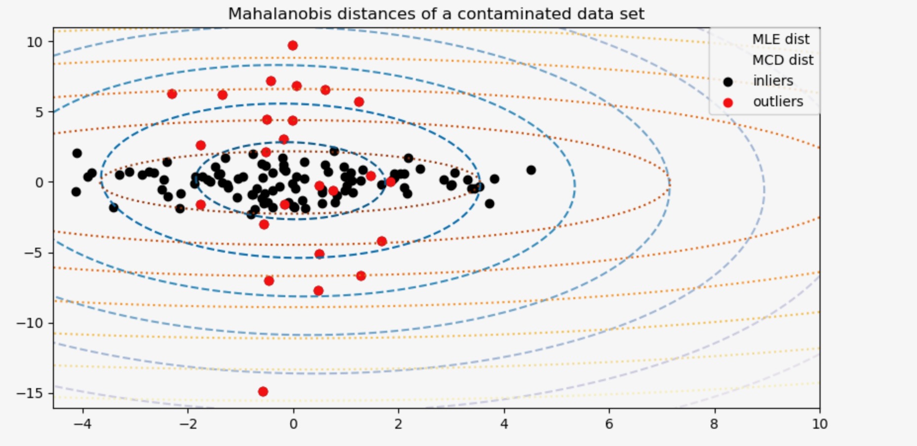

　最後に、外れ値を識別するためのMCDに基づくマハラノビス距離の能力を強調します。私たちはマハラノビス距離の立方根(cubic root)を取ります。およそ正規分布(WilsonとHilfertyに提案された)に分離し、その後ボックスプロットに内部と外れ値の値を図示します。外れ値サンプルの分布は、ロバストMCDに基づくマハラノビス距離のために、内部サンプルの分布からもっと区別されます。

fig, (ax1, ax2) = plt.subplots(1, 2)
plt.subplots_adjust(wspace=0.6)

# Calculate cubic root of MLE Mahalanobis distances for samples
emp_mahal = emp_cov.mahalanobis(X - np.mean(X, 0)) ** (0.33)
# Plot boxplots
ax1.boxplot([emp_mahal[:-n_outliers], emp_mahal[-n_outliers:]], widths=0.25)
# Plot individual samples
ax1.plot(
    np.full(n_samples - n_outliers, 1.26),
    emp_mahal[:-n_outliers],
    "+k",
    markeredgewidth=1,
)
ax1.plot(np.full(n_outliers, 2.26), emp_mahal[-n_outliers:], "+k", markeredgewidth=1)
ax1.axes.set_xticklabels(("inliers", "outliers"), size=15)
ax1.set_ylabel(r"$\sqrt[3]{\rm{(Mahal. dist.)}}$", size=16)
ax1.set_title("Using non-robust estimates\n(Maximum Likelihood)")

# Calculate cubic root of MCD Mahalanobis distances for samples
robust_mahal = robust_cov.mahalanobis(X - robust_cov.location_) ** (0.33)
# Plot boxplots
ax2.boxplot([robust_mahal[:-n_outliers], robust_mahal[-n_outliers:]], widths=0.25)
# Plot individual samples
ax2.plot(
    np.full(n_samples - n_outliers, 1.26),
    robust_mahal[:-n_outliers],
    "+k",
    markeredgewidth=1,
)
ax2.plot(np.full(n_outliers, 2.26), robust_mahal[-n_outliers:], "+k", markeredgewidth=1)
ax2.axes.set_xticklabels(("inliers", "outliers"), size=15)
ax2.set_ylabel(r"$\sqrt[3]{\rm{(Mahal. dist.)}}$", size=16)
ax2.set_title("Using robust estimates\n(Minimum Covariance Determinant)")

plt.show()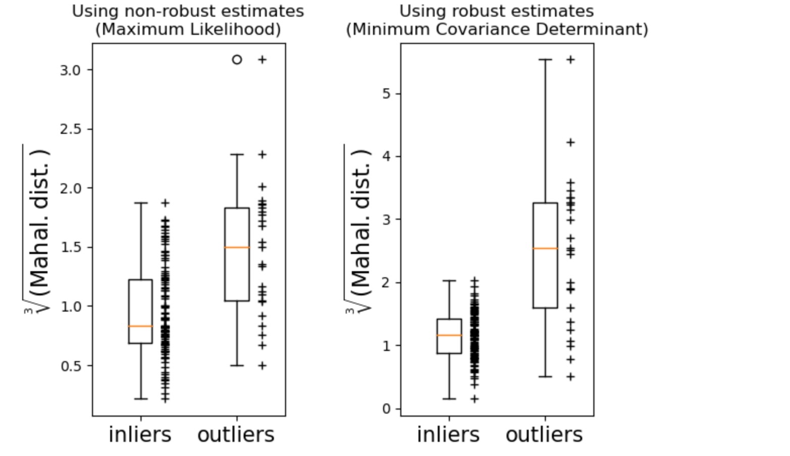