カーネル密度推定は、カーネル関数K(u)を用いて未知の確率密関数を推定する過程です。ヒストグラムは、幾分恣意的な領域のデータポイントの数を計数しますが、カーネル密度推定は、全てのデータポイントのカーネル関数の合計として定義される関数です。カーネル関数は典型的には以下の性質を示します。
- 対称性 K(u) = K(-u)のような
- 正規化 ∮ ー♾️♾️ K(u) du = 1
- 単調減少 u > 0の時に K'(u) < 0
- 期待値がゼロ E[ K ] = 0
カーネル密度のより詳しい情報は、Wikipediaの Kernel density estimation を参照してください。
単変量カーネル密度推定は sm.nonparametric.KDEUnivariateに実装されています。この例では、以下のことを示します。
- 基本的な使用法、推定の適合の仕方
- bw引数を使ったカーネルのバンド幅の変位の影響
- kernel引数を使った色々なカーネル関数の利用
%matplotlib inline
import numpy as np
from scipy import stats
import statsmodels.api as sm
import matplotlib.pyplot as plt
from statsmodels.distributions.mixture_rvs import mixture_rvs
単変量の例
位置を−1と1にしたふたつの正規分布を混合した:二つのモードの分布を作ります。
# Location, scale and weight for the two distributions
dist1_loc, dist1_scale, weight1 = -1, 0.5, 0.25
dist2_loc, dist2_scale, weight2 = 1, 0.5, 0.75

# Sample from a mixture of distributions
obs_dist = mixture_rvs(
    prob=[weight1, weight2],
    size=250,
    dist=[stats.norm, stats.norm],
    kwargs=(
        dict(loc=dist1_loc, scale=dist1_scale),
        dict(loc=dist2_loc, scale=dist2_scale),
    ),
)
密度推定のための最も簡単なノンパラメトリック技術はヒストグラムです。
fig = plt.figure(figsize=(12, 5))
ax = fig.add_subplot(111)

# Scatter plot of data samples and histogram
ax.scatter(
    obs_dist,
    np.abs(np.random.randn(obs_dist.size)),
    zorder=15,
    color="red",
    marker="x",
    alpha=0.5,
    label="Samples",
)
lines = ax.hist(obs_dist, bins=20, edgecolor="k", label="Histogram")

ax.legend(loc="best")
ax.grid(True, zorder=-5)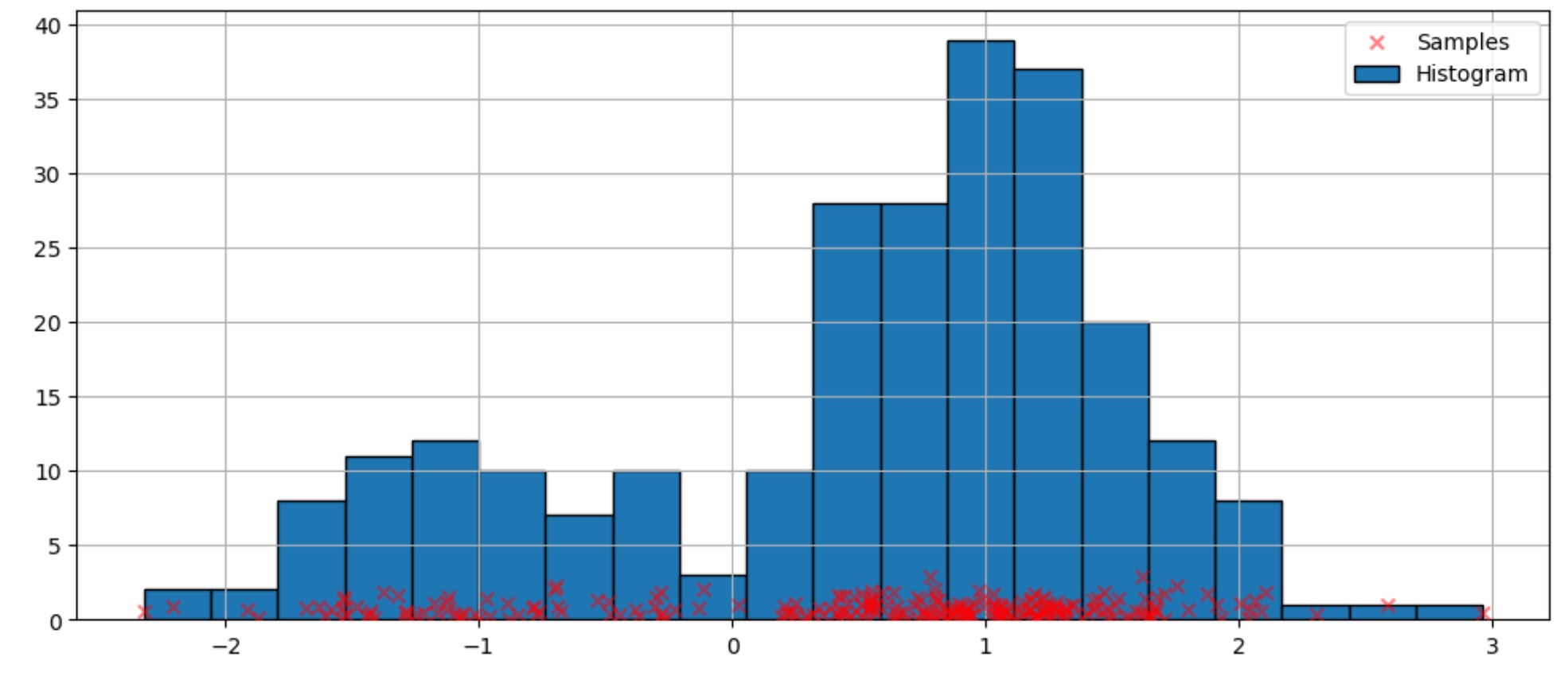
デフォルト引数の適合
上のヒストグラムは不連続です。連続確率密度関数を計算するために、カーネル密度推定を使うことができます。
私たちは、KDEUnivariateを使って単変量カーネル密度推定を初期化します。
kde = sm.nonparametric.KDEUnivariate(obs_dist)
kde.fit()  # Estimate the densities
<statsmodels.nonparametric.kde.KDEUnivariate at 0x15b27bdc0>私たちは、適合の図と同じように真の分布を表します。
fig = plt.figure(figsize=(12, 5))
ax = fig.add_subplot(111)

# Plot the histogram
ax.hist(
    obs_dist,
    bins=20,
    density=True,
    label="Histogram from samples",
    zorder=5,
    edgecolor="k",
    alpha=0.5,
)

# Plot the KDE as fitted using the default arguments
ax.plot(kde.support, kde.density, lw=3, label="KDE from samples", zorder=10)

# Plot the true distribution
true_values = (
    stats.norm.pdf(loc=dist1_loc, scale=dist1_scale, x=kde.support) * weight1
    + stats.norm.pdf(loc=dist2_loc, scale=dist2_scale, x=kde.support) * weight2
)
ax.plot(kde.support, true_values, lw=3, label="True distribution", zorder=15)

# Plot the samples
ax.scatter(
    obs_dist,
    np.abs(np.random.randn(obs_dist.size)) / 40,
    marker="x",
    color="red",
    zorder=20,
    label="Samples",
    alpha=0.5,
)

ax.legend(loc="best")
ax.grid(True, zorder=-5)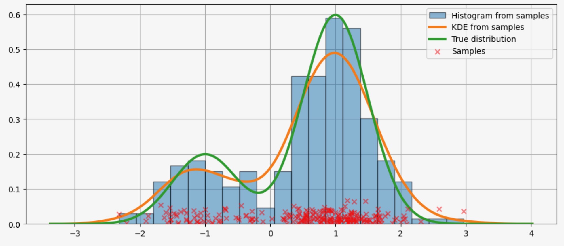
上のコードでは、デフォルトの引数が使われています。私たちはここで見るように、カーネルのバンド幅を変えることができます。
bw引数を使ったバンド幅の変更
カーネルのバンド幅はbw引数を使って適合させることができます。以下の例では、bw=0.2のバンド幅で、データがうまく適合するようです。
fig = plt.figure(figsize=(12, 5))
ax = fig.add_subplot(111)

# Plot the histogram
ax.hist(
    obs_dist,
    bins=25,
    label="Histogram from samples",
    zorder=5,
    edgecolor="k",
    density=True,
    alpha=0.5,
)

# Plot the KDE for various bandwidths
for bandwidth in [0.1, 0.2, 0.4]:
    kde.fit(bw=bandwidth)  # Estimate the densities
    ax.plot(
        kde.support,
        kde.density,
        "--",
        lw=2,
        color="k",
        zorder=10,
        label="KDE from samples, bw = {}".format(round(bandwidth, 2)),
    )

# Plot the true distribution
ax.plot(kde.support, true_values, lw=3, label="True distribution", zorder=15)

# Plot the samples
ax.scatter(
    obs_dist,
    np.abs(np.random.randn(obs_dist.size)) / 50,
    marker="x",
    color="red",
    zorder=20,
    label="Data samples",
    alpha=0.5,
)

ax.legend(loc="best")
ax.set_xlim([-3, 3])
ax.grid(True, zorder=-5)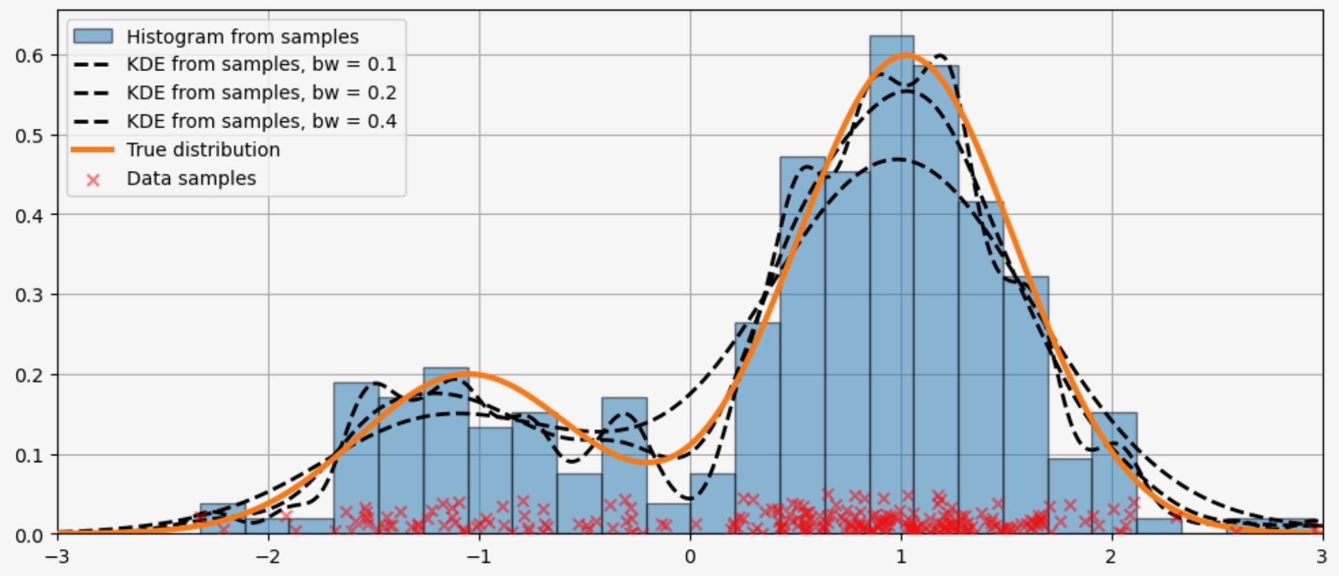
カーネル関数の比較
上の例では、ガウシアンカーネルが使われました。数種の他のカーネルが利用できます。
from statsmodels.nonparametric.kde import kernel_switch

list(kernel_switch.keys())
['gau', 'epa', 'uni', 'tri', 'biw', 'triw', 'cos', 'cos2', 'tric']利用できるカーネル関数
# Create a figure
fig = plt.figure(figsize=(12, 5))

# Enumerate every option for the kernel
for i, (ker_name, ker_class) in enumerate(kernel_switch.items()):

    # Initialize the kernel object
    kernel = ker_class()

    # Sample from the domain
    domain = kernel.domain or [-3, 3]
    x_vals = np.linspace(*domain, num=2 ** 10)
    y_vals = kernel(x_vals)

    # Create a subplot, set the title
    ax = fig.add_subplot(3, 3, i + 1)
    ax.set_title('Kernel function "{}"'.format(ker_name))
    ax.plot(x_vals, y_vals, lw=3, label="{}".format(ker_name))
    ax.scatter([0], [0], marker="x", color="red")
    plt.grid(True, zorder=-5)
    ax.set_xlim(domain)

plt.tight_layout()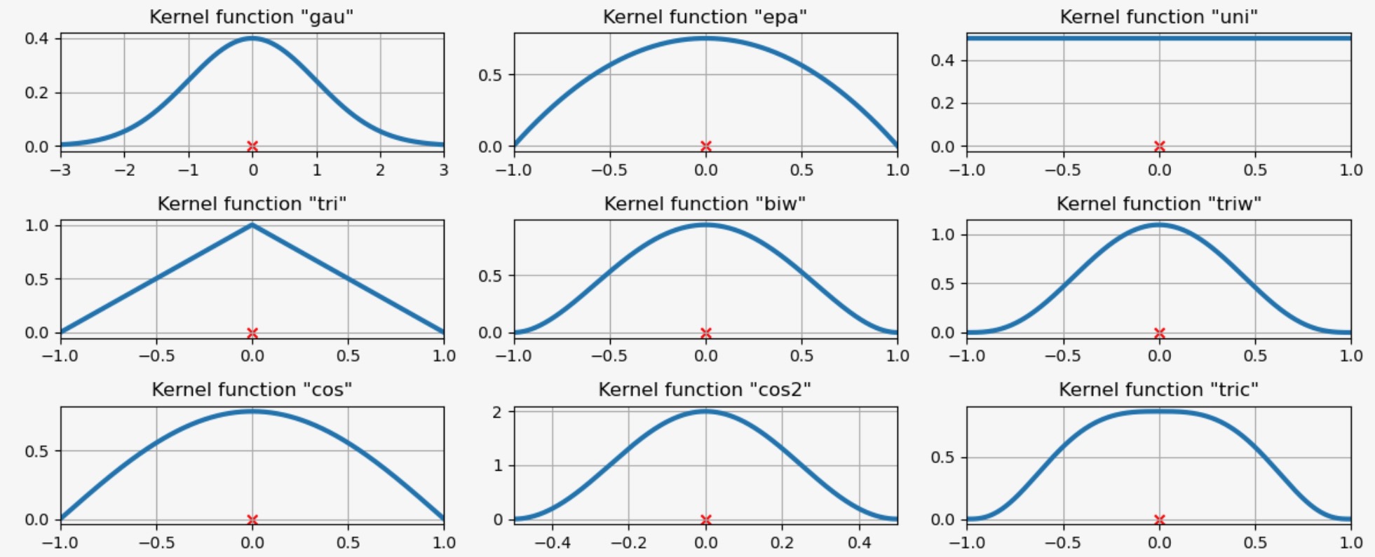
3つのデータポイントで利用できるカーネル関数
私たちは、ここでどのようにカーネル密度推定が三つの等間隔のデータポイントに適合するか検証します。
# Create three equidistant points
data = np.linspace(-1, 1, 3)
kde = sm.nonparametric.KDEUnivariate(data)

# Create a figure
fig = plt.figure(figsize=(12, 5))

# Enumerate every option for the kernel
for i, kernel in enumerate(kernel_switch.keys()):

    # Create a subplot, set the title
    ax = fig.add_subplot(3, 3, i + 1)
    ax.set_title('Kernel function "{}"'.format(kernel))

    # Fit the model (estimate densities)
    kde.fit(kernel=kernel, fft=False, gridsize=2 ** 10)

    # Create the plot
    ax.plot(kde.support, kde.density, lw=3, label="KDE from samples", zorder=10)
    ax.scatter(data, np.zeros_like(data), marker="x", color="red")
    plt.grid(True, zorder=-5)
    ax.set_xlim([-3, 3])

plt.tight_layout()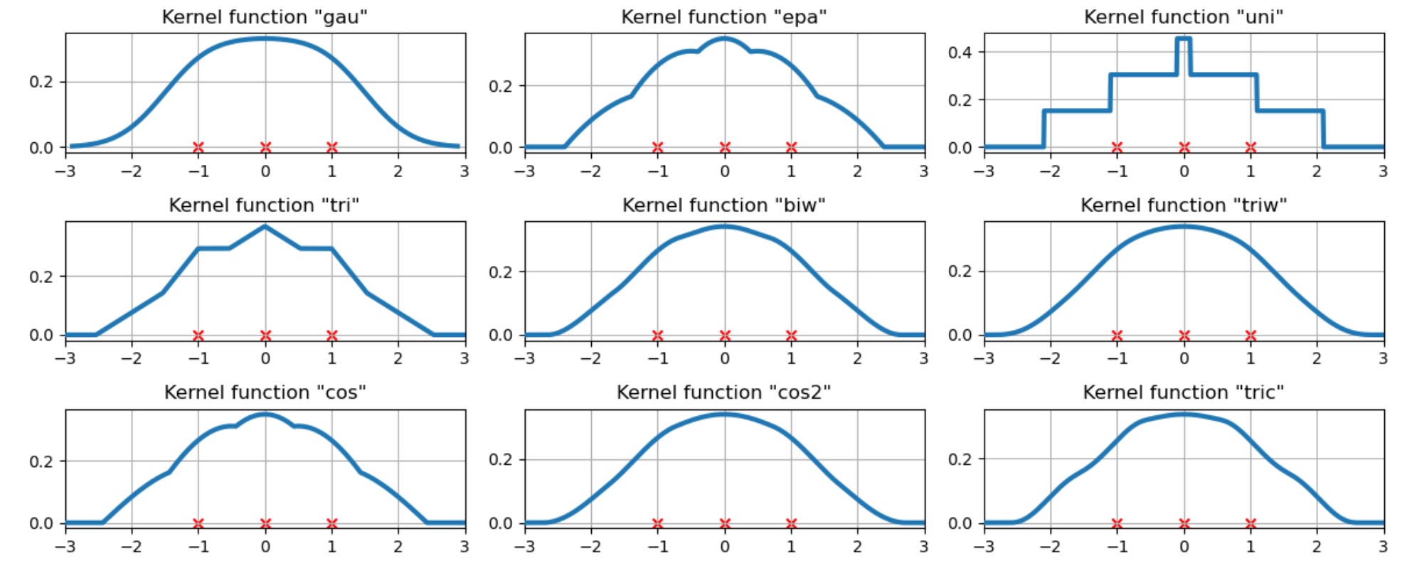
もっと困難なケース
適合はいつも完全なわけではありません。以下の困難なケースの例を見てください。
obs_dist = mixture_rvs(
    [0.25, 0.75],
    size=250,
    dist=[stats.norm, stats.beta],
    kwargs=(dict(loc=-1, scale=0.5), dict(loc=1, scale=1, args=(1, 0.5))),
)
kde = sm.nonparametric.KDEUnivariate(obs_dist)
kde.fit()<statsmodels.nonparametric.kde.KDEUnivariate at 0x15b7fcb20>fig = plt.figure(figsize=(12, 5))
ax = fig.add_subplot(111)
ax.hist(obs_dist, bins=20, density=True, edgecolor="k", zorder=4, alpha=0.5)
ax.plot(kde.support, kde.density, lw=3, zorder=7)
# Plot the samples
ax.scatter(
obs_dist,
np.abs(np.random.randn(obs_dist.size)) / 50,
marker="x",
color="red",
zorder=20,
label="Data samples",
alpha=0.5,
)
ax.grid(True, zorder=-5)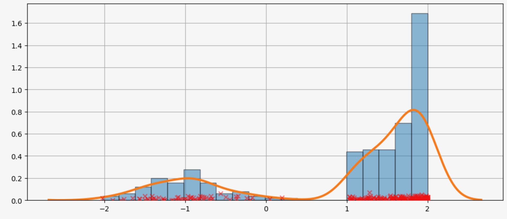
KDEは分布
KDEは分布なので、私たちは次のような属性とメソッドにアクセスすることができます。
- entropy
- evaluate
- cdf
- icdf
- sf
- cumhazard
obs_dist = mixture_rvs(
    [0.25, 0.75],
    size=1000,
    dist=[stats.norm, stats.norm],
    kwargs=(dict(loc=-1, scale=0.5), dict(loc=1, scale=0.5)),
)
kde = sm.nonparametric.KDEUnivariate(obs_dist)
kde.fit(gridsize=2 ** 10)
<statsmodels.nonparametric.kde.KDEUnivariate at 0x15b7d5e70>kde.entropy1.314324140492138kde.evaluate(-1)array([0.18085886])累積分布、その逆累積分布、生存関数
fig = plt.figure(figsize=(12, 5))
ax = fig.add_subplot(111)

ax.plot(kde.support, kde.cdf, lw=3, label="CDF")
ax.plot(np.linspace(0, 1, num=kde.icdf.size), kde.icdf, lw=3, label="Inverse CDF")
ax.plot(kde.support, kde.sf, lw=3, label="Survival function")
ax.legend(loc="best")
ax.grid(True, zorder=-5)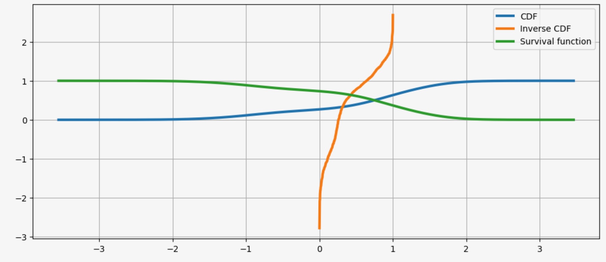
を用いて未知の確率密関数を推定する過程です。ヒストグラムは、幾分恣意的な領域のデータポイントの数を計数しますが、カーネル密度推定は、全てのデータポイントのカー )