ここに、経済データのトレンドとサイクルを分離する三つの方法を考えます。私たちがもっている時系列データytを考えます。基本の考えは、それを二つの成分に分解することです。
yt = μt + ηtここで、μtはトレンド、またはレベル、ηt は、サイクル成分を表します。このケースでは、私たちは、μt は、時間の決定関数でなくランダム変数なので、確率的なトレンドを考えます。ふたつのメソッドは”観測されない成分”に分類されます。3番目のメソッドは、一般的なHodrick-Prescott(HP)フィルターです。例えば、Harvey とJaeger(1993) に一致します。私たちは、これらのモデルが同様の分解で生み出されることがわかります。
このノートブックは、これらのモデルに、U.S失業率のサイクルからトレンドを分離するために、これらのモデルに適用することを示します。
%matplotlib inlineimport numpy as np
import pandas as pd
import statsmodels.api as sm
import matplotlib.pyplot as pltfrom pandas_datareader.data import DataReader
endog = DataReader('UNRATE', 'fred', start='1954-01-01')
endog.index.freq = endog.index.inferred_freqHodrick-Prescott(HP) フィルター
最初の方法は、Hodrick-Prescottフィルターです。それは、とても前進する方法でデータ系列に適用することができます。ここで、私たちは、パラメータλ=129600を規定します。なぜなら、失業率は月次で観測されます。
hp_cycle, hp_trend = sm.tsa.filters.hpfilter(endog, lamb=129600)観測されない成分とARIMAモデル(UC-ARIMA)
次のメソッドは、観測されない成分のモデルです、ここで、トレンドはランダムウォークととしてモデル化され、サイクルはARIMAモデルー特に、ここではAR(4)モデルでモデル化されます。その時系列過程は次のように書けます。

ここで、Φ(L)は、AR(4)遅延式、εtとνtはホワイトノイズです。
mod_ucarima = sm.tsa.UnobservedComponents(endog, 'rwalk', autoregressive=4)
# Here the powell method is used, since it achieves a
# higher loglikelihood than the default L-BFGS method
res_ucarima = mod_ucarima.fit(method='powell', disp=False)
print(res_ucarima.summary())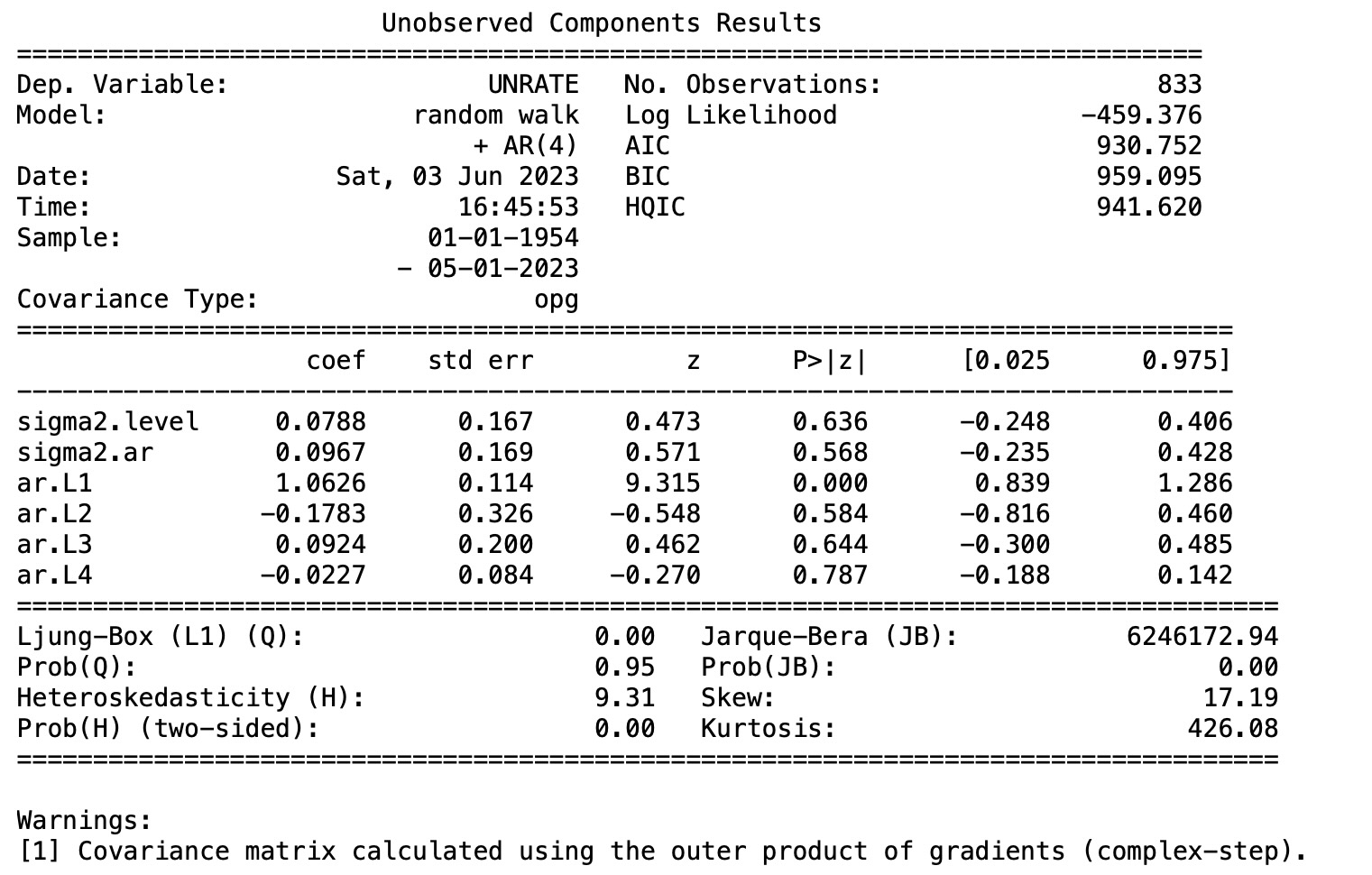
観測されない成分と確率サイクル(UC)
最後の方法も、観測されない成分モデルです。しかし、サイクルは明確にモデル化されます。
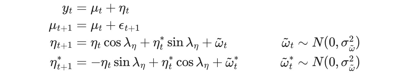
mod_uc = sm.tsa.UnobservedComponents(
    endog, 'rwalk',
    cycle=True, stochastic_cycle=True, damped_cycle=True,
)
# Here the powell method gets close to the optimum
res_uc = mod_uc.fit(method='powell', disp=False)
# but to get to the highest loglikelihood we do a
# second round using the L-BFGS method.
res_uc = mod_uc.fit(res_uc.params, disp=False)
print(res_uc.summary())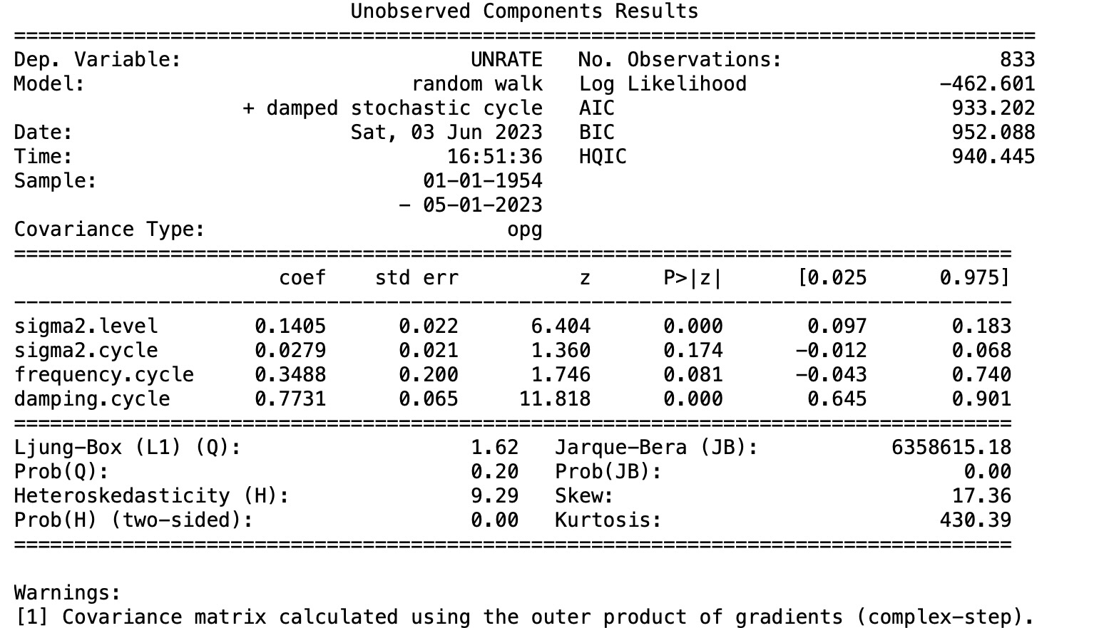
グラフィカル比較
これらのモデルの各出力は、トレンド成分μt の推定とサイクル成分ηt の推定です。HPフィルターのトレンド成分は、観測されない成分のモデルより幾らか不安定ですが、トレンドとサイクルの推定の性質はよく似ています。これは、失業率の変動の相対的なモードが、一時的なサイクル変動よりもトレンドの影響下で変化していると考えられることを意味しています。
fig, axes = plt.subplots(2, figsize=(13,5));
axes[0].set(title='Level/trend component')
axes[0].plot(endog.index, res_uc.level.smoothed, label='UC')
axes[0].plot(endog.index, res_ucarima.level.smoothed, label='UC-ARIMA(2,0)')
axes[0].plot(hp_trend, label='HP Filter')
axes[0].legend(loc='upper left')
axes[0].grid()

axes[1].set(title='Cycle component')
axes[1].plot(endog.index, res_uc.cycle.smoothed, label='UC')
axes[1].plot(endog.index, res_ucarima.autoregressive.smoothed, label='UC-ARIMA(2,0)')
axes[1].plot(hp_cycle, label='HP Filter')
axes[1].legend(loc='upper left')
axes[1].grid()

fig.tight_layout();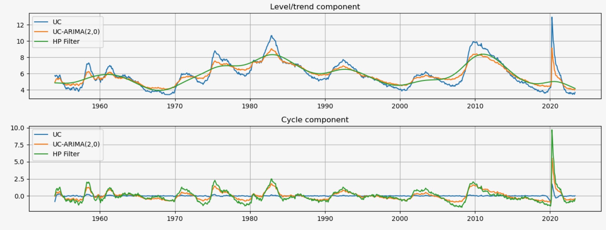