因果探索の共通のタスクは、なぜ仮定したまたは再構築した因果ネットワークが理解され、訂正し、正当化することです。ここに私たちは、データセットの遅延相関構造を説明するモデルを構築するために、どのようにグラフの推定を使うことができるかを示します。ステップは次のようになります。
- 因果グラフの推定(マルコフ同値類の)
- もし、マルコフ同値類が、一つ以上のメンバーを持つならば、自動的に類の一つのメンバーを選択します。
- 線形構造因果モデルを、グラフから取った親に適合させます
- 残りのノイズの共分散行列を推定します。
- ノイズ構造とともに、線形ガウス構造モデルを構築し、データとして同じサンプルサイズの多くの実現値を生成します。
- 生成したデータの(集団の平均と信頼区間)遅延相関とオリジナルデータの遅延相関を示します。
# Imports
import numpy as np
import matplotlib
from matplotlib import pyplot as plt
%matplotlib inline

import tigramite
from tigramite import data_processing as pp
from tigramite.toymodels import structural_causal_processes as toys

from tigramite.toymodels import surrogate_generator

from tigramite import plotting as tp
from tigramite.pcmci import PCMCI
from tigramite.independence_tests.parcorr import ParCorr
from tigramite.models import Models, Prediction

import math
import sklearn
from sklearn.linear_model import LinearRegression
0. 同時に発生する従属性と任意の事例過程を生成
np.random.seed(14)     # Fix random seed
lin_f = lambda x: x
links_coeffs = {0: [((0, -1), 0.7, lin_f)],
                1: [((1, -1), 0.8, lin_f), ((0, -1), 0.3, lin_f)],
                2: [((2, -1), 0.5, lin_f), ((0, -2), -0.5, lin_f)],
                3: [((3, -1), 0., lin_f)], #, ((4, -1), 0.4, lin_f)],
                4: [((4, -1), 0., lin_f), ((3, 0), 0.5, lin_f)], #, ((3, -1), 0.3, lin_f)],
                }
T = 200     # time series length
# Make some noise with different variance, alternatively just noises=None
noises = np.array([(1. + 0.2*float(j))*np.random.randn((T + int(math.floor(0.2*T))))
                   for j in range(len(links_coeffs))]).T

data, _ = toys.structural_causal_process(links_coeffs, T=T, noises=noises, seed=14)
T, N = data.shape

# For generality, we include some masking
# mask = np.zeros(data.shape, dtype='int')
# mask[:int(T/2)] = True
mask=None

# Initialize dataframe object, specify time axis and variable names
var_names = [r'$X^0$', r'$X^1$', r'$X^2$', r'$X^3$', r'$X^4$']
dataframe = pp.DataFrame(data,
                         mask=mask,
                         datatime = {0:np.arange(len(data))},
                         var_names=var_names)
tp.plot_timeseries(dataframe=dataframe); plt.show()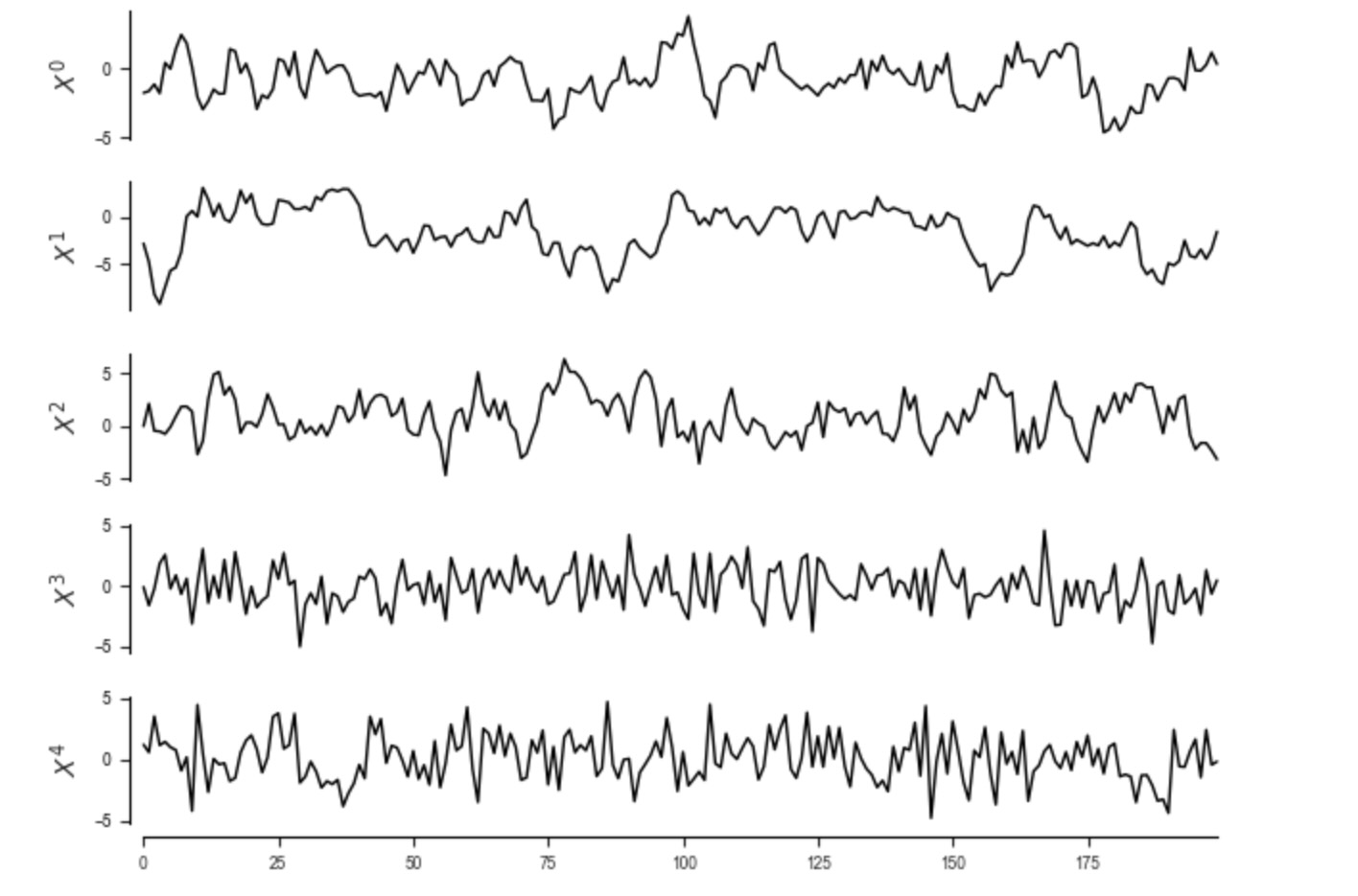
ここで、遅延相関行列をみてみましょう。私たちは、それを説明する構造因果モデルを見つけたいのです。
tau_max = 10
parcorr = ParCorr(significance='analytic',
#                   mask_type='y'
                 )
pcmci = PCMCI(
    dataframe=dataframe,
    cond_ind_test=parcorr,
    verbosity=0)
original_correlations = pcmci.get_lagged_dependencies(tau_max=tau_max, val_only=True)['val_matrix']
lag_func_matrix = tp.plot_lagfuncs(val_matrix=original_correlations, setup_args={'var_names':var_names,
                                    'x_base':5, 'y_base':.5}); plt.show()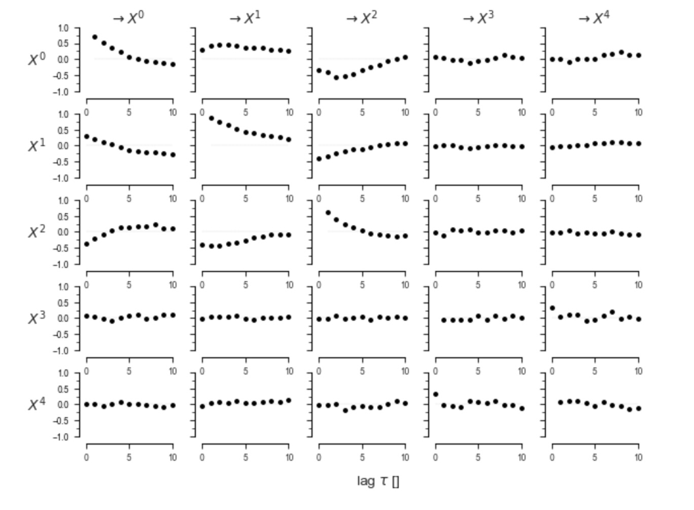
1. 因果グラフ(マルコフ同値類)の推定
ここで私たちは、 妥当なtau_maxとpc_alphaの設定で、PCMCI+を実行します。もちろん、推定モデルは、これらのパラメータに僅かに依存しています。
results = pcmci.run_pcmciplus(tau_max=tau_max, pc_alpha=0.01)
tp.plot_graph(results['graph']); plt.show()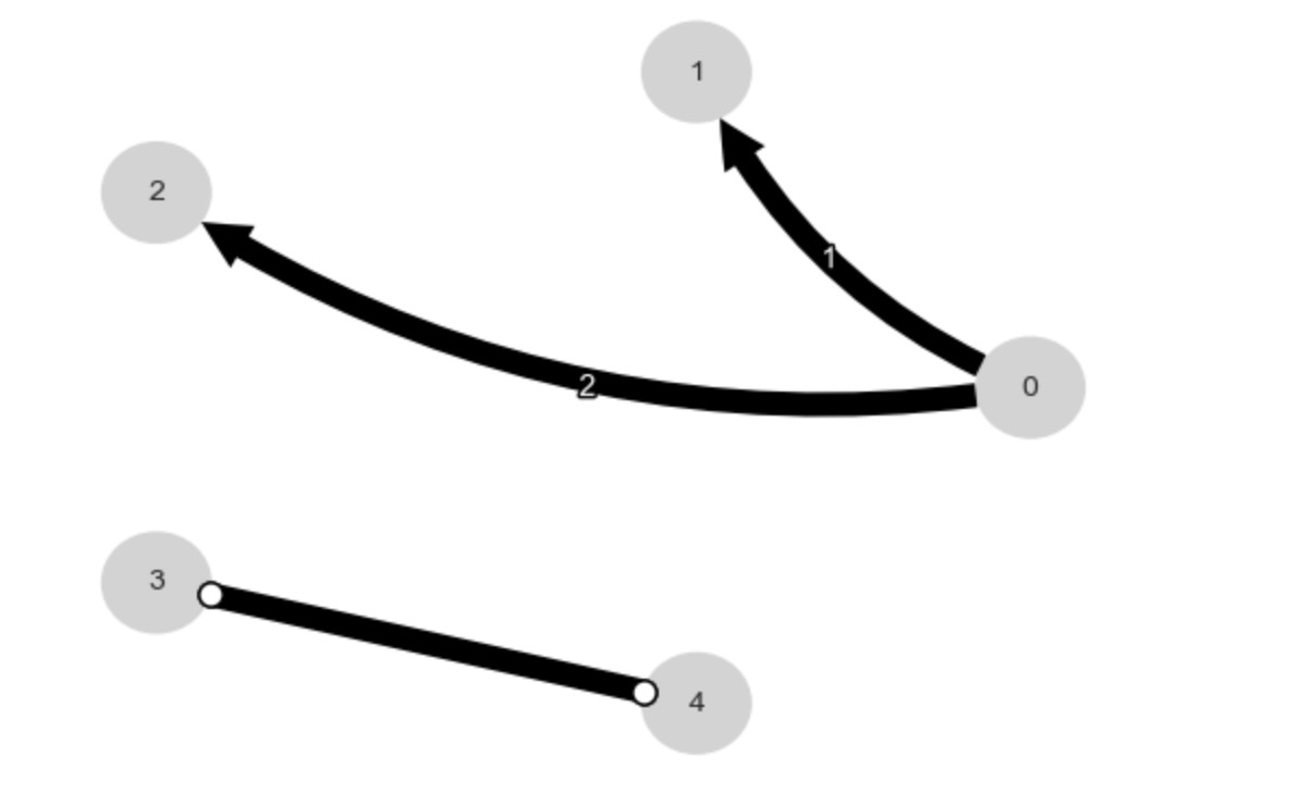
2. もし、マルコフ同値類が一つ以上のメンバーを持つならば、(中心のないエッジの発生)、自動的に類の一つを選択
PCMCI+の結果は、CPDAG(方向性のないエッジ)です。私たちは、クラスからある関数を使って、一つのDAGメンバーを選択します。
# First create order that is based on some feature of the variables
# to avoid order-dependence of DAG, i.e., it should not matter
# in which order the variables appear in dataframe
# Here we use the sum of absolute val_matrix values incident at j
val_matrix = results['val_matrix']
variable_order = np.argsort(
                    np.abs(val_matrix).sum(axis=(0,2)))[::-1]

# Transform conflicting links to unoriented links as a hack, might not work...
graph = results['graph']
graph[graph=='x-x'] = 'o-o'
dag = pcmci._get_dag_from_cpdag(
                cpdag_graph=graph,
                variable_order=variable_order)

tp.plot_graph(dag); plt.show()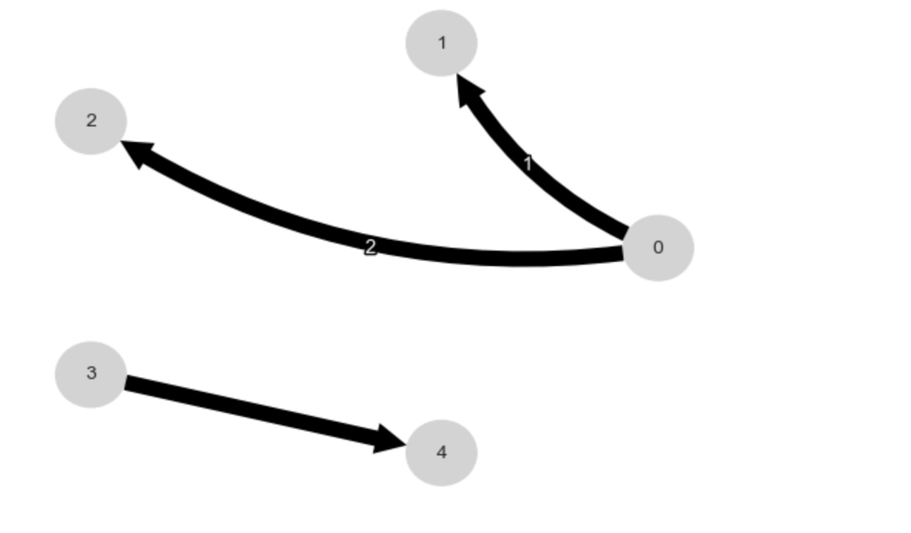
以下のステップは、モジュールtoymodels.surrogate_generatorの関数generate_linear_model_from_dataで全て包まれます。
3. 線形構造因果モデルをグラフから取得した因果上の親に適合する
Model()を呼ぶ予測クラスを使用。
4. 残りのノイズの共分散行列を推定する
予測クラスを使用
5. ノイズ構造とともに線形ガウスクラスを構築
parents = toys.dag_to_links(dag)
print(parents)
{0: [(0, -1)], 1: [(0, -1), (1, -1)], 2: [(0, -2), (2, -1)], 3: [], 4: [(3, 0)]}ここで、データと同じサンプルサイズの多くの実現値を生成する
realizations = 100

generator = surrogate_generator.generate_linear_model_from_data(dataframe, parents, tau_max, realizations=realizations,
                generate_noise_from='covariance')
datasets = {}
for r in range(realizations):
    datasets[r] = next(generator)
6. 生成データの遅延相関とオリジナルデータの遅延相関を表示する
correlations = np.zeros((realizations, N, N, tau_max + 1))
for r in range(realizations):
    pcmci = PCMCI(
        dataframe=pp.DataFrame(datasets[r]),
        cond_ind_test=ParCorr(),
        verbosity=0)
    correlations[r] = pcmci.get_lagged_dependencies(tau_max=tau_max, val_only=True)['val_matrix']
# Get mean and 5th and 95th quantile
correlation_mean = correlations.mean(axis=0)
correlation_interval = np.percentile(correlations, q=[5, 95], axis=0)# Plot lag functions of mean and 5th and 95th quantile together with original correlation in one plot
lag_func_matrix = tp.setup_matrix(N=N, tau_max=tau_max, x_base=5, figsize=(10, 10), var_names=var_names)
lag_func_matrix.add_lagfuncs(val_matrix=correlation_mean, color='black')
lag_func_matrix.add_lagfuncs(val_matrix=correlation_interval[0], color='grey')
lag_func_matrix.add_lagfuncs(val_matrix=correlation_interval[1], color='grey')
lag_func_matrix.add_lagfuncs(val_matrix=original_correlations, color='red')
lag_func_matrix.savefig(name=None)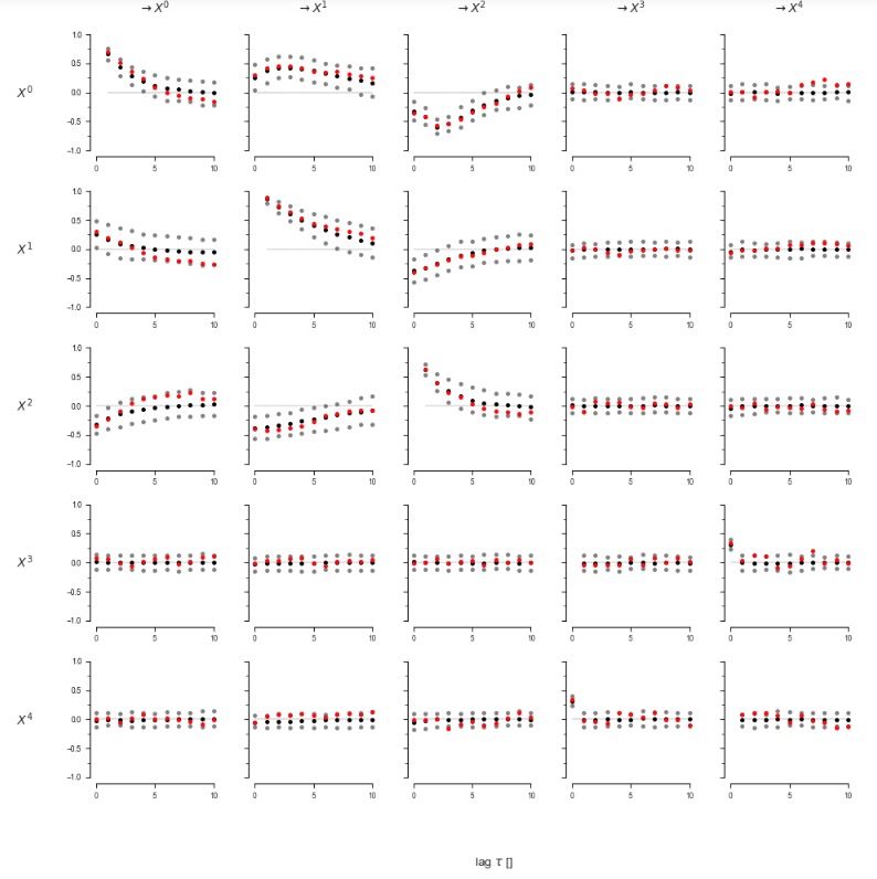
赤のオリジナル遅延関数は、おおよそ生成データの相関の90%(グレイ)の範囲にあります。ほら、これは、再構築された因果グラフからのそれらは、オリジナルデータの全体の遅延相関構造をよく説明することができるので、同じリンク(そしてノイズ構造と係数を推定した)の線形ガウスモデルを意味します。
最後に、私たちは、(たたみ込んだ)相関グラフを表示することができます。
pcmci = PCMCI(
    dataframe=dataframe,
    cond_ind_test=parcorr,
    verbosity=0)
original_correlations_pvals = pcmci.get_lagged_dependencies(tau_max=tau_max)['p_matrix']
tp.plot_graph(graph=original_correlations_pvals<=0.01); plt.show()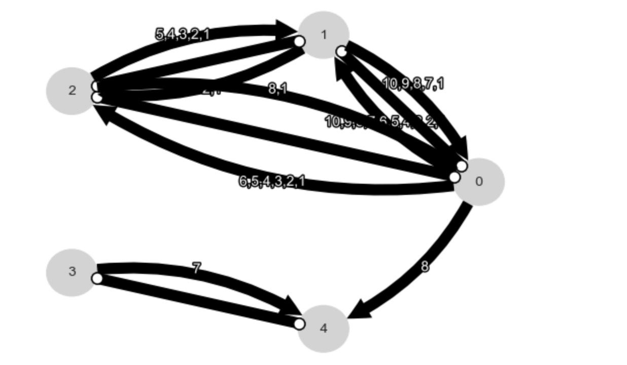