TIGRAMITEは時系列分析Pythonモジュールです。PCMCIフレームワークを基礎にした離散、連続時系列からグラフィカルモデル(条件独立グラフ)を再構築し、結果の高品質の図を生成します。
以下のNature Review Earth and Environment論文は、一般的な時系列のための因果推論の概要を提供します。
https://github.com/jakobrunge/tigramite/blob/master/tutorials/Runge_Causal_Inference_for_Time_Series_NREE.pdf
このチュートリアルは、関数PCMCI.run_sliding_window_ofを説明します。それは、多変量時系列を超えてスライディング・スライディング上で、全てのPCMCI因果探索メソッドが実行できる、便利な関数です。
# Imports
import numpy as np
import matplotlib
from matplotlib import pyplot as plt
%matplotlib inline
## use `%matplotlib notebook` for interactive figures
# plt.style.use('ggplot')

import tigramite
from tigramite import data_processing as pp
from tigramite.toymodels import structural_causal_processes as toys
from tigramite import plotting as tp
from tigramite.pcmci import PCMCI
from tigramite.independence_tests.parcorr import ParCorr
設定
PCMCIとその派生は多変量時系列データから時系列グラフを再構築することができます。重要な前提になる仮定は、因果のステーショナリティーで、例えば、条件独立性関係は、時間上でステーショナリーです。従って、因果リンクの存在と欠如は、ステーショナリーです。ときに、因果関係は、特定の期間内でだけステーショナリーであることがわかるでしょう。例えば、私たちは、夏と冬で異なる因果関係を観察するかもしれません。このケースは、対応するチュートリアルで議論したようにマスキング機能によって取り扱われます。
run_sliding_window_ofに実装されたスライディング・ウィンドウ分析では、一方で、私たちは、時系列上をスライドする時間ウインドウの順序とは分離して、因果グラフの推定を導きます。それは、method, window_step s、および、window_length wによって与えられます。私たちは、各時間ウィンドウ{Xt}t=s-i s-i+w-1のサンプル上で、順番にメソッドを実行させます。
以下で、二つの潜在的な使用法を議論します。
使用ケース1:時間変化因果ダイナミクス
このケースで、私たちは、基礎になる確率過程Xi=(Xt1,…,XtN)が、時間変異の因果構造を持つことを仮定します。これは、機能の依存性、因果の親、ノイズ分布に影響します。従って、私たちは、以下の構造因果モデルを仮定します。

ここで、ftjは、平凡でない従属性を引数Pt(Xtj)とηtjに持つ任意の関数です。最後の変数は、排他性(i ≠ j)と連続性(t'≠ t)を持つ独立の動的ノイズの、以下のある分布Dtを表します。以前との相違は、三つの変数ftj,P(Xtj),そしてDtすべては、ここでは、時間に依存しています。
もちろん、もしこの時間従属性が何らかの方法で制限されないならば、そのとき因果関係は識別することができません。以下の例で、私たちは、遅い混乱させる(confounder)Uによって規定された、ゆっくりとした変異について考慮します。
np.random.seed(42)
N = 4
T = 100000
data = np.random.randn(T, N)
datatime = np.arange(T)

# Simple unobserved confounder U that smoothly changes causal relations
U = np.cos(np.arange(T)*0.00005) #+ 0.1*np.random.randn(T)
c = 0.8
for t in range(1, T):
    if U[t] >= 0:
        data[t, 0] += 0.4*data[t-1, 0]
        data[t, 1] += 0.5*data[t-1, 1] + 0.4*U[t]*data[t-1, 0]
        data[t, 2] += 0.6*data[t-1, 2] + data[t, 0]
    else:
        data[t, 2] += 0.6*data[t-1, 2]
        data[t, 0] += 0.4*data[t-1, 0] + 0.4*data[t, 2]
        data[t, 1] += 0.5*data[t-1, 1] + 0.4*U[t]*data[t-1, 0]
    data[t, 3] = U[t]

# Initialize dataframe object, specify variable names
var_names = [r'$X^{%d}$' % j for j in range(N-1) ] + [r'$U$']
dataframe_plot = pp.DataFrame(data, var_names=var_names)
tp.plot_timeseries(dataframe_plot); plt.show()

# For the analysis we use only the observed data
dataframe = pp.DataFrame(data[:,:3], var_names=var_names[:-1])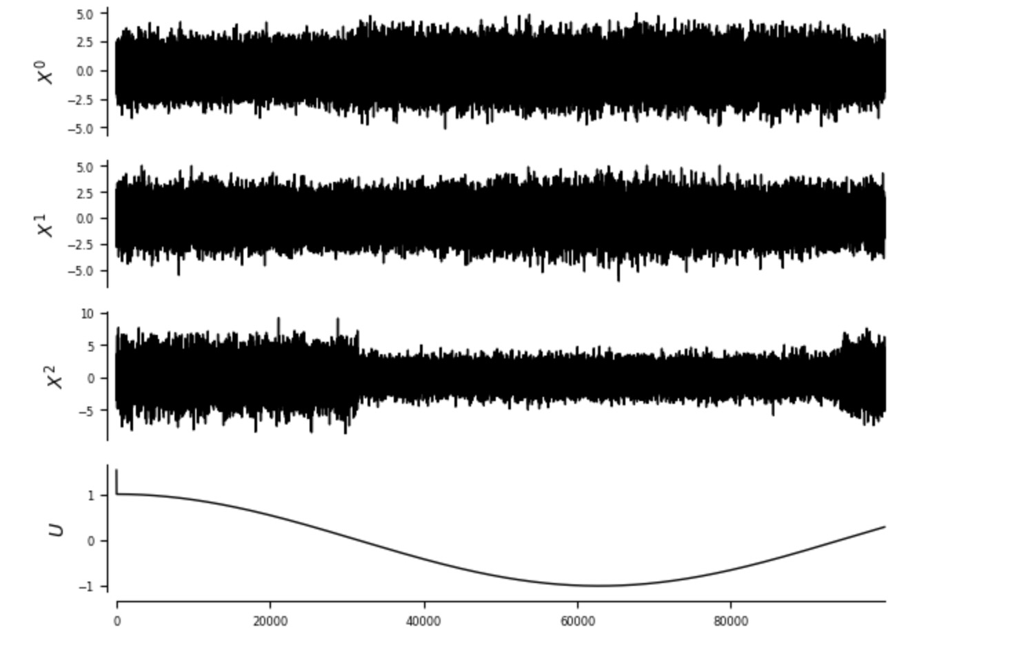
あなたがデータ生成過程からわかるように、Uは、Xt-10 ->Xt1 の因果リンクの強度と符号、そして加えて、Xt0とXt2のあいだで同時に発生するリンクの因果の方向、が変化します。私たちは、観測していないUがわからないことと、X0,X1,X2からだけでデータフレームを構築することを仮定します。
私たちは、ここで、method='run_pcmciplus',window_step=1000とwindow_length=10000に設定した run_sliding_window_ofを実行します。'run_pcmciplus'への追加の引数は、method_argsを使って渡されます。もちろん、ウィンドウは、オーバーラップすることを選択しても良いでしょう。
window_step=10000
window_length=10000
method='run_pcmciplus'
method_args={'tau_min':0, 'tau_max':2, 'pc_alpha':0.01}
conf_lev = 0.95
cond_ind_test = ParCorr(significance='analytic')

# Init
pcmci = PCMCI(
    dataframe=dataframe,
    cond_ind_test=cond_ind_test,
    verbosity=0)
# Run
results = pcmci.run_sliding_window_of(method=method,
                                    method_args=method_args,
                                    window_step=window_step,
                                    window_length=window_length,
conf_lev = conf_lev) run_sliding_window_ofはエントリー'summary_results'と'window_results'のdictionaryを返します。最初の人るは、2番目の使用ケースで議論します。result['window_results']はここで、標準のPCMCIplus分析として、同じ結果のエントリーを含みます。しかし、各自は、全てのスライディングウィンドウの結果のリストです。以下、私たちは、graphとval_matrixに焦点を当て、そしてそれらを時系列上で整列させて視覚化します。
graphs = results['window_results']['graph']
val_matrices = results['window_results']['val_matrix']
n_windows = len(graphs)

mosaic = [['data %s' %j for i in range(n_windows)] for j in range(N)]
for n in range(N):
    mosaic.append(['graph %s' %i for i in range(n_windows)])
# print(mosaic)
fig, axs = plt.subplot_mosaic(mosaic = mosaic, figsize=(20, 10))

for j in range(N):
    ax = axs['data %s' %j]
    ax.axhline(0., color='grey')
    if j ==3:
        ax.fill_between(x=datatime, y1=-1, y2=1, where=datatime <= window_length, color='grey', alpha=0.3)

    if j == 3: color = 'black'
    else: color = 'blue'
    ax.plot(datatime, data[:,j], color=color)
#     axs['data %s' %j].axis('off') # xaxis.set_ticklabels([])
    for loc, spine in ax.spines.items():
        if loc != 'left':
            spine.set_color("none")

    ax.xaxis.set_ticks([])
    ax.set_xlim(0., T)
    ax.set_ylabel(var_names[j])

for w in range(n_windows):
    if w == 0: show_colorbar=True
    else: show_colorbar = False
    tp.plot_graph(graphs[w], val_matrix=val_matrices[w], show_colorbar=show_colorbar,
                  fig_ax=(fig, axs['graph %s' %w]))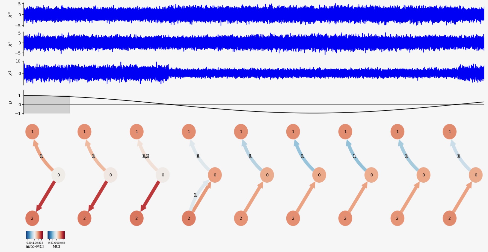
見てわかるように、ここに、九つのスライディングウィンドウがあります。(長さは、U時系列の灰色のバーで示されます。推定されたように、時間を超えて強度とXt-10->Xt1の因果リンクの符号と強度、加えて、Xt0とXt2の変化の間で同時に発生するリンクの因果検出は変化します)
私たちは、val_matiricesからXt-10 -> Xt1の因果リンクのリンク強度の値を抽出します。
fig = plt.figure(figsize=(4, 2))
ax = fig.add_subplot(111)
ax.plot(list(range(n_windows)), val_matrices[:, 0, 1, 1])
ax.axhline(color='black')
ax.set_xlabel("Sliding window")
ax.set_ylabel("Link Strength")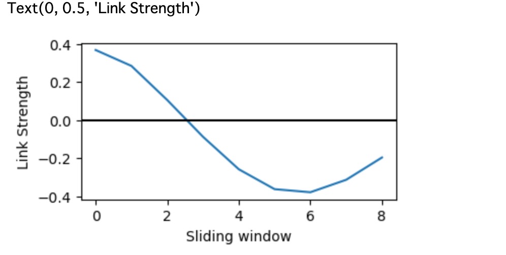
使用ケース2:ゆっくりと変化するconfounderによるステーショナリー因果関係
このケースでは、私たちは、Xiの間でXt=(Xt1,…,XtN)の間でSCMが、時間上でステーショナリーであることを仮定します。例えば、fj, P(Xtj), Dは、時間に依存しませんが、外部にゆっくりと変化するconfounderを追加します。(もちろん、真のSCMは、このconfounderを含みます)
np.random.seed(42)
N = 4
T = 10000
data = np.random.randn(T, N)
datatime = np.arange(T)
# Simple unobserved confounder U that smoothly changes causal relations
U = np.cos(np.arange(T)*0.0005) #+ 0.1*np.random.randn(T)
c = 3.
for t in range(1, T):
    data[t, 2] += 0.6*data[t-1, 2] + c*U[t]
    data[t, 0] += 0.4*data[t-1, 0] + 0.4*data[t, 2] + c*U[t]
    data[t, 1] += 0.5*data[t-1, 1] + 0.05*data[t-1, 0] + c*U[t]
    data[t, 3] = U[t]

# Initialize dataframe object, specify variable names
var_names = [r'$X^{%d}$' % j for j in range(N-1) ] + [r'$U$']
dataframe_plot = pp.DataFrame(data, var_names=var_names)
tp.plot_timeseries(dataframe_plot); plt.show()

# For the analysis we use only the observed data
dataframe = pp.DataFrame(data[:,:3], var_names=var_names[:-1])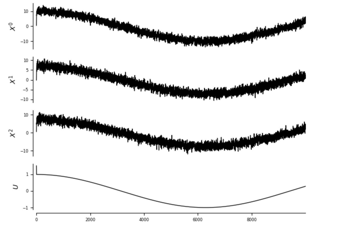
私たちは、時系列全体とスライディングウィンドウの両方の分析を実行します。
window_step=1000
window_length=1000
method='run_pcmciplus'
method_args={'tau_min':0, 'tau_max':2, 'pc_alpha':0.01}
conf_lev = 0.95
cond_ind_test = ParCorr(significance='analytic')

# Init
pcmci = PCMCI(
    dataframe=dataframe,
    cond_ind_test=cond_ind_test,
    verbosity=0)
# Run
results = pcmci.run_sliding_window_of(method=method,
                                    method_args=method_args,
                                    window_step=window_step,
                                    window_length=window_length,
                                    conf_lev = conf_lev)
results_alldata = pcmci.run_pcmciplus(**method_args)
強力な非観測のconfoundingは、それらを依存させる全ての変数のトレンドを含みます。従って、もし私たちが、時間フレームの全体を分析するならば、私たちは、ほぼ全ての接続したグラフを取得します。
tp.plot_graph(graph=results_alldata['graph'], val_matrix=results_alldata['val_matrix']); plt.show()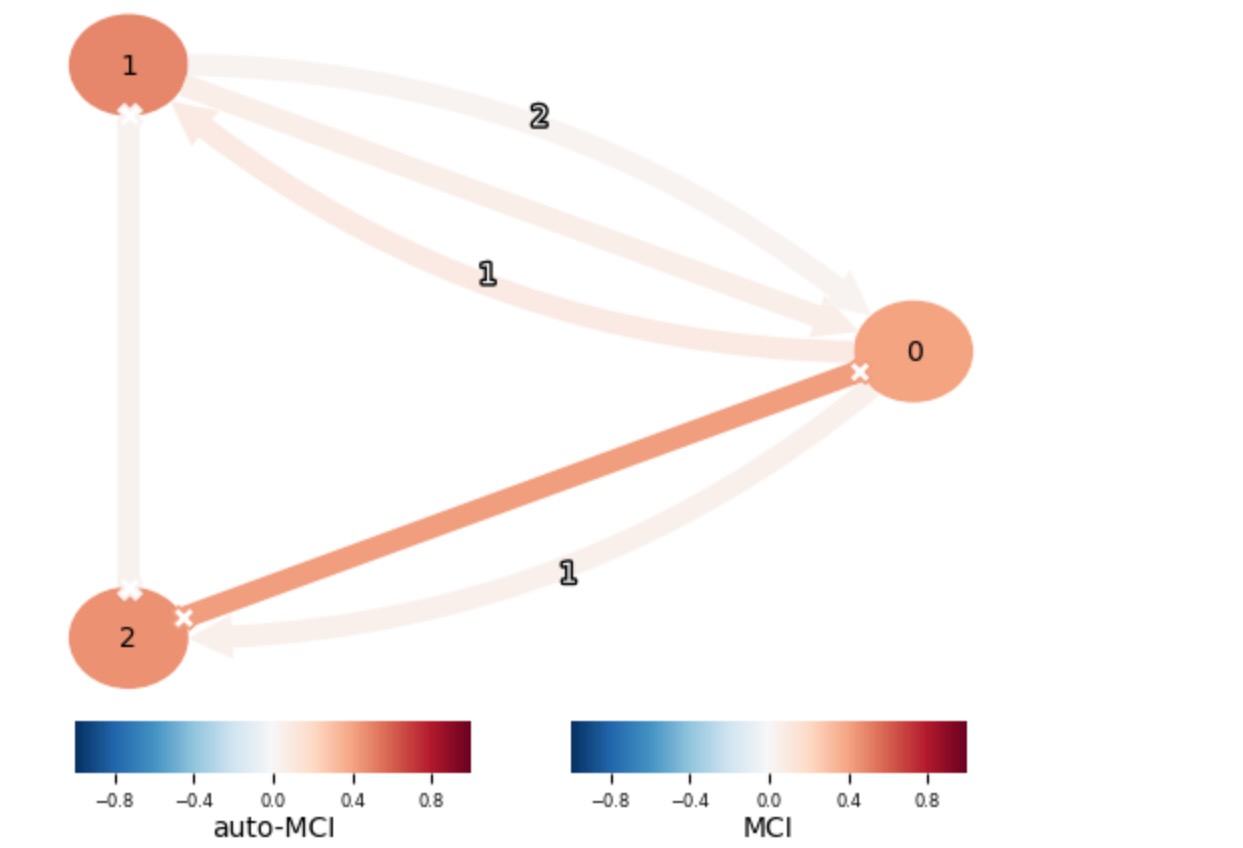
一方で、非観測のconfounder各スライディングウィンドウは、一定であることが仮定されます。従って、混乱させられることはありません。
graphs = results['window_results']['graph']
val_matrices = results['window_results']['val_matrix']
n_windows = len(graphs)

mosaic = [['data %s' %j for i in range(n_windows)] for j in range(N)]
for n in range(N):
    mosaic.append(['graph %s' %i for i in range(n_windows)])
# print(mosaic)
fig, axs = plt.subplot_mosaic(mosaic = mosaic, figsize=(20, 10))

for j in range(N):
    ax = axs['data %s' %j]
    ax.axhline(0., color='grey')
    if j ==3:
        ax.fill_between(x=datatime, y1=-1, y2=1, where=datatime <= window_length, color='grey', alpha=0.3)

    if j == 3: color = 'black'
    else: color = 'blue'
    ax.plot(datatime, data[:,j], color=color)
#     axs['data %s' %j].axis('off') # xaxis.set_ticklabels([])
    for loc, spine in ax.spines.items():
        if loc != 'left':
            spine.set_color("none")

    ax.xaxis.set_ticks([])
    ax.set_xlim(0., T)
    ax.set_ylabel(var_names[j])

for w in range(n_windows):
    if w == 0: show_colorbar=True
    else: show_colorbar = False
    tp.plot_graph(graphs[w], val_matrix=val_matrices[w], show_colorbar=show_colorbar,
                  fig_ax=(fig, axs['graph %s' %w]))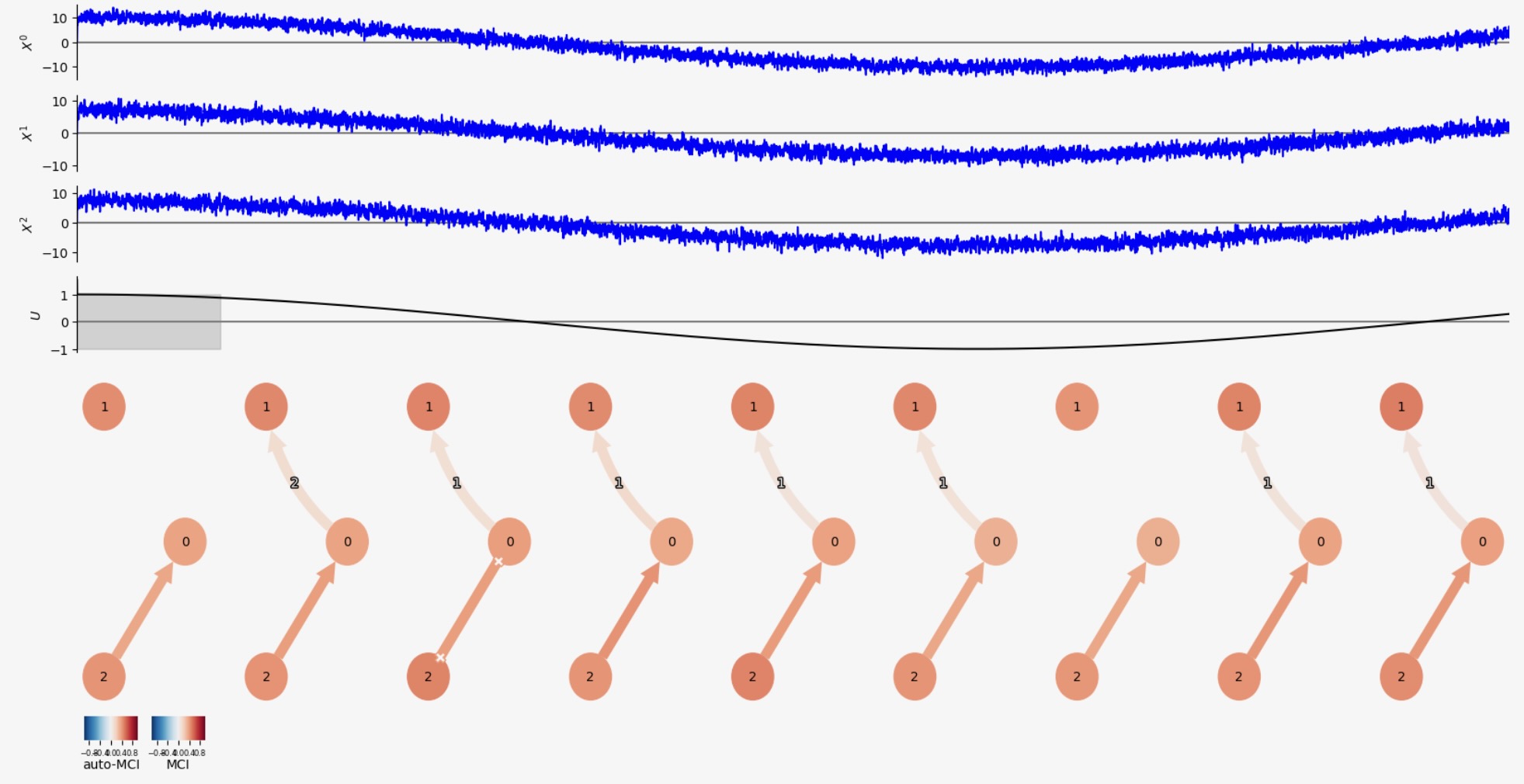
ここで、グラフは、時間上でむしろステーショナリーです。effectively_srationary SCMの仮定によって私たちは、'summary_results'の統計結果を考慮するでしょう。'most_frequent_links'は、各エントリーが、スライディングウィンドウの間で、最も頻繁に発生するリンクを含む、リンク""の欠如を含むグラフを含みます。'link_frequency'は、リンクが発生するところのスライディングウィンドウの変化を含みます。最後に、'val_matrix_mean'は、全ての時間ウィンドウを覆う平均したテスト統計値を含みます。これら三つの特徴は、plot_graphを使って視覚化されます。
注記:テスト静的値(例えば、部分相関)は、従属性のstrengthの性質の直感を与えるかもしれない。しかし適当な因果結果分析は、CausalEffectsクラスを参照してください。
tp.plot_graph(graph=results['summary_results']['most_frequent_links'],
              val_matrix=results['summary_results']['val_matrix_mean'],
             link_width=results['summary_results']['link_frequency'])
print('most_frequent_links')
print(results['summary_results']['most_frequent_links'].squeeze())
print('link_frequency')
print(results['summary_results']['link_frequency'].squeeze())
most_frequent_links
[[['' '-->' '']
['' '-->' '']
['<--' '' '']]
[['' '' '']
['' '-->' '']
['' '' '']]
[['-->' '' '']
['' '' '']
['' '-->' '']]]
link_frequency
[[[1. 1. 0.88888889]
[1. 0.66666667 0.88888889]
[0.88888889 1. 1. ]]
[[1. 1. 1. ]
[1. 1. 1. ]
[1. 1. 1. ]]
[[0.88888889 1. 1. ]
[1. 1. 1. ]
[1. 1. 1. ]]]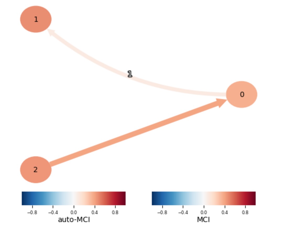
ここで、X0->X1のリンクは弱く、そして、ウィンドウの小さな変化を検出するだけです。
を再構築し、結果の高品質の図を生成します。 )